
MORE QUESTIONS
CONTACT US
FAQ BUY
What probe series does Sensepeek offer, what are the differences between them, and what is their frequency range? ▼
Sensepeek offers a variety of probe series, each tailored for different measurement needs and frequency ranges from DC up to 6 GHz.
SP10:
Frequency Range: Up to 10 MHz 1:1 probe with dupont connector, ultra thin PCB - design.
Features: Basic handsfree probes suitable for low-frequency measurements, packed together with test wires for connection directly to a logic analyzer, multimeter, or your preferred tool. Perfect for I2C, UART, CAN-bus, etc. No more soldering wires to connect your probe or complicated tools to set up; just position the probe needle on any test point or component in the signal path and release. The minimalist design and spring-loaded test needle allow for simultaneous measurements on fine pitch components and nearby signals. The probe is steady yet flexible, designed for instant measurements or total hands-free operations with your multimeter or logic analyzer. It comes with a powerful magnet in the base for easy placement and repositioning.
Learn more
SQ Series Overview:
The SQ series of handsfree probes from Sensepeek feature a lower center of gravity for enhanced stability compared to the original SP series. Insulated and designed for both handheld and handsfree operation, these probes include improved ground options, probe tip protection, longer cables, and support for oscilloscopes with automatic scaling. They make instant measurements or long triggering sessions a breeze. The beloved features such as exchangeable fine-pitch spring-tipped test needles and color-coded cable holders make traditional probes obsolete. The perfectly balanced length and weight ensure optimal use with PCB holders and the powerful magnet in the base allows for easy placement and repositioning.
SQ10:
Frequency Range: Up to 10 MHz 1:1 probe with dupont connector, insulated design
Complete handsfree SQ10 probe packed together with test wires for connection directly to a logic analyzer, multimeter, or your preferred tool. Perfect for I2C, UART, CAN-bus, etc.
Learn more
SQ100:
Frequency Range: Up to 100 MHz, BNC connector, CATII 300V RMS
Features: One complete handsfree 100 MHz oscilloscope probe.
Learn more
SQ200:
Frequency Range: Up to 200 MHz, BNC connector, CATII 300V RMS
Features: One complete handsfree 200 MHz oscilloscope probe, read out - pin on BNC with support for oscilloscopes with automatic scaling.
Learn more
SQ350:
Frequency Range: Up to 350 MHz, BNC connector, CATII 300V RMS
Features: One complete handsfree 350 MHz oscilloscope probe, read out - pin on BNC with support for oscilloscopes with automatic scaling.
Learn more
SQ500:
Frequency Range: Up to 500 MHz, BNC connector, CATII 300V RMS
Features: One complete handsfree 500 MHz oscilloscope probe, read out - pin on BNC with support for oscilloscopes with automatic scaling.
Learn more
SQG Series Overview:
Introducing the SQG series of high-frequency handsfree probes from Sensepeek, designed for both AC and DC applications. With exceptionally low probe tip capacitance, the SQG series minimizes signal distortion and is ideal for sensitive circuits. They ensure crisp, precise measurements even at high data rates, making them perfect for RF traces and fast data interfaces. The SQG series includes exchangeable fine-pitch spring-tipped test needles and dual ground options, offering unmatched adaptability. These probes are compatible with any measurement instrument featuring a 50 Ω input impedance and are packaged in a specially designed case for safe transport. Ideal for engineers seeking precision and ease of use in high-frequency measurements.
SQG15-AC:
Frequency Range: Up to 1.5 GHz
Features: Probe tip impedance of 500 Ω; usable data rate exceeding 3 Gbps, making it ideal for high-speed signal measurements; remarkably low probe tip capacitance of less than 1.36 pF, preventing capacitive loading; flat frequency response (+/- 0.5dB) from 1.0 kHz to 700 MHz; return loss for probed line, typically -26 dB to -11 dB in the range 0 - 1.5 GHz.
Learn more
SQG15-DC:
Frequency Range: Up to 1.5 GHz
Features: Probe tip impedance of 500 Ω; usable data rate exceeding 6 Gbps, making it ideal for high-speed signal measurements; continues voltage up to 16 V; flat frequency response (+/- 0.5dB) from DC to 800 MHz; return loss for probed line, typically -26 dB to -11.5 dB in the range 0 - 1.5 GHz.
Learn more
SQG30-AC:
Frequency Range: Up to 3.0 GHz
Features: Probe tip impedance of 500 Ω; usable data rate exceeding 6 Gbps, making it ideal for high-speed signal measurements; continues voltage up to 15 V; flat frequency response (+/- 0.5dB) from DC to 2.75 GHz; up to 2 GHz with single GND and above 3 GHz with the dual GND clip.
Learn more
SQG30-DC:
Frequency Range: Up to 3.0 GHz
Features: Probe tip impedance of 333 Ω; usable data rate exceeding 12 Gbps, making it ideal for high-speed signal measurements; remarkably low probe tip capacitance of less than 0.69 pF, preventing capacitive loading; flat frequency response (+/- 0.5dB) from 1.15 kHz to 5.4 GHz; max ringing 0.065 dB at 3 GHz and 0.15 dB at 6 GHz.
Learn more
SQG60-AC:
Frequency Range: Up to 6.0 GHz
Features: Probe tip impedance of 333 Ω; usable data rate exceeding 12 Gbps, making it ideal for high-speed signal measurements; remarkably low probe tip capacitance of less than 0.69 pF, preventing capacitive loading; transition time < 52 ps, 10% - 90%; continues voltage up to 13 V.
Learn more
SQG60-DC:
Frequency Range: Up to 6.0 GHz
Features: Probe tip impedance of 333 Ω; usable data rate exceeding 12 Gbps, making it ideal for high-speed signal measurements; remarkably low probe tip capacitance of less than 0.69 pF, preventing capacitive loading; transition time < 52 ps, 10% - 90%; continues voltage up to 13 V.
Learn more
I have an xxx MHz oscilloscope. Which probe should I buy? ▼
Simple answer: Buy the highest frequency probe you can afford.
Detailed answer: Oscilloscope and Probe: Combining Bandwidth for Optimal Results.
The bandwidth of an oscilloscope is a critical factor in its ability to capture and display signals accurately. As the frequency of the signal increases, the oscilloscope’s ability to represent the signal with precision diminishes. Bandwidth refers to the range of frequencies that the oscilloscope can measure without significant signal distortion. This specification is typically defined by the IEEE 1057 standard, which describes bandwidth as the point where the amplitude of a sine wave input is reduced by 3 dB, or about 30%, from its original value at lower frequencies. Essentially, at the oscilloscope’s bandwidth limit, the signal will only display 70.7% of its true amplitude, making it an important consideration for high-frequency measurements.
A common question among oscilloscope users is whether they can measure a high-frequency signal, such as 93 MHz clock, using a 100 MHz oscilloscope with a 100 MHz passive probe. On the surface, this seems reasonable, but it often leads to confusion. This is because manufacturers rarely discuss the combined bandwidth of the oscilloscope and the probe, known as "system bandwidth."
Both the oscilloscope and the probe have individual bandwidth specifications that indicate when the signal’s amplitude will be attenuated by 3 dB. However, the combined bandwidth, or system bandwidth, is not simply the sum or average of these values.
For example, using a 100 MHz oscilloscope with a 100 MHz probe often results in a system bandwidth of around 70 MHz, not 100 MHz.
Looking at the 93 MHz clock signal with the 100 MHz oscilloscope and the 100 MHz probe, you’ll see a sine wave on the oscilloscope instead of a square wave. However, if you had used the same 100 MHz oscilloscope with a 350 MHz probe, you would see a square wave.This is due to the Gaussian filters commonly used in oscilloscope design, which smooth the response but also lower the effective bandwidth.
In oscilloscopes, the Gaussian filter acts as a low-pass filter. This means that it allows low-frequency components of the signal to pass through while attenuating higher frequencies. The bandwidth of the filter determines how much high-frequency content is removed. For example, a narrow bandwidth Gaussian filter will only allow slow, smooth changes in the signal to pass through, eliminating high-frequency noise and signal components.
The Gaussian response filter follows a predictable roll-off, and the system bandwidth can be calculated using the square root of the sum of the squares formula.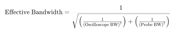
Where:
Oscilloscope BW is the bandwidth of the oscilloscope
Probe BW is the bandwidth of the probe
This formula calculates the combined effective bandwidth of the oscilloscope and probe. The overall bandwidth of the measurement system will be lower than the smallest bandwidth of either the oscilloscope or the probe.
System BW for probe and oscilloscopes with Gaussian filter
In contrast, a Brickwall filter in an oscilloscope is a type of frequency response filter characterized by its sharp cutoff at a specified bandwidth. Unlike traditional filters, which gradually attenuate frequencies above their cutoff point, a Brickwall filter sharply transitions from the passband to the stopband, resembling a vertical wall. This design ensures maximal flatness within the passband, allowing the filter to maintain a consistent amplitude for signals within the specified frequency range without distortion.
The defining feature of a Brickwall filter is its abrupt attenuation of frequencies beyond the cutoff frequency, effectively minimizing aliasing and unwanted signals in the measured data. This makes Brickwall filters particularly valuable in high-frequency applications where precise signal integrity is crucial, such as in digital oscilloscopes and high-speed data acquisition systems. By cutting off high-frequency noise, they help prevent distortion of the measured signal.
In practical terms, a Brickwall filter's response can be visualized as a steep slope beyond its cutoff frequency, which maintains very little signal amplitude beyond this point. This contrasts with Gaussian filters, which have a more gradual roll-off. When using a Brickwall filter, the overall system bandwidth of an oscilloscope and probe combination can be calculated simply as the minimum of their respective bandwidths, since the Brickwall filter does not allow any additional bandwidth margin.
In summary, Brickwall filters are essential for ensuring accurate measurements in high-frequency applications, providing a clear distinction between the signal of interest and noise.
While it is rare to see Brickwall filters in oscilloscopes with lower bandwidth ratings, such as 100 MHz, this distinction is critical when operating at higher frequencies. In cases where a Brickwall filter is present, the system bandwidth is effectively the same as the lowest individual component's bandwidth. For example, a 200 MHz oscilloscope and a 350 MHz probe has a system BW of 200 MHz, where a Gaussian oscilloscope has an effective BW of 163 MHz.
Where:
Oscilloscope BW is the bandwidth of the oscilloscope
Probe BW is the bandwidth of the probe
It's important to note that many oscilloscopes and probes have some margin in their bandwidth ratings, often exceeding the specified value slightly. For example, a 200 MHz oscilloscope may be capable of measuring signals up to 220 MHz and the probe up to 250 MHz before significant attenuation occurs.
The type of filter in an oscilloscope, whether Gaussian or Brickwall, can be determined by calculating its rise time. For scopes with Gaussian filters, the rise time is typically calculated using a constant of 0.35, while scopes with a Brickwall response use a constant closer to 0.45. By dividing the rise time by the appropriate constant, the effective bandwidth of the oscilloscope can be established. For example, if a 350 MHz oscilloscope’s data sheet indicates a rise time of 1 ns, the calculation would be: 0.35 / 1 ns = 350 MHz. This indicates that the oscilloscope likely features a Gaussian filter.
Understanding these principles is essential when working with high-frequency signals. By taking into account system bandwidth and the type of filter response, engineers can ensure more accurate and reliable measurements, avoiding common pitfalls when operating oscilloscopes near their bandwidth limits.
FAQ MEASURE
Why should I use a short GND lead for high frequency measurements? ▼
Impact of Grounding and Ground Leads
A key factor in probe performance is the grounding system. Probes typically include a ground clip, designed to provide a low-impedance return path for the signal, placed at the front of the ground tube housing the front end. However, the inductance introduced by the ground lead can significantly distort measurements, especially at higher frequencies.
For instance, a typical ground clip wire introduces approximately 1 nH of inductance per millimeter, meaning a 100 mm ground lead adds around 100 nH of inductance to the measurement setup. This inductance can cause peaking in the frequency response, distort the transient response, and make it difficult to accurately capture fast signal transitions.
Although using a long ground lead may seem convenient for signal identification, it can drastically reduce the probe’s effective bandwidth. A ground lead between 100 to 150 mm can cause even a standard 10:1 probe to exhibit significant amplification above 10-20 MHz, leading to excessive signal ringing and an artificially high voltage level. This may result in poor hardware adjustment decisions, as users might believe the signal requires damping or other corrective measures, when the real issue lies in improper grounding.
High-bandwidth probes often include low-inductance grounding accessories, such as coaxial connections or short ground pins, to minimize inductance and preserve signal integrity. In high-frequency applications, ensuring proper grounding is crucial for accurate measurements and avoiding misleading data, which could lead to unnecessary hardware modifications.
Unfortunately some manufacturers provide performance data only achievable with soldered-in accessories that are not part of the standard probe kit or inflate their performance claims by using solid surrounding ground adapters directly inserted into the test-instruments during the -3dB measurement. Resulting in boosted probe-data-sheets and poor performance fo the end user.
Reputable oscilloscope probe manufacturers design probes with bandwidths and performance specifications measured using the shortest possible ground lead included in the package. Using a method similar to what the end user will do during a measurement, to guarantee that the end user will experience the best performance.
What is the maximum voltage rating for the SQ-series probes? ▼
The SQ-series probes have a maximum voltage rating of 300V CAT II, making them suitable for a wide range of electronic measurements.
What is the maximum voltage rating for the SP-series probes? ▼
The SP-series probes have a maximum voltage rating of +/-60 V DC, 30 V AC RMS, +/-42.4 V pk max
Can the GND needle be adjusted? ▼
Yes, follow the guide here
Adjusting the Ground Needle for Perfect Probe Fit
How do I make the handsfree arm stable? ▼
Measuring with the probe
1. Position the arm in 45 degree angle
2. Lift the probe in the probe grip
3. Compress the needle to the measuring target
4. Release the probe grip gently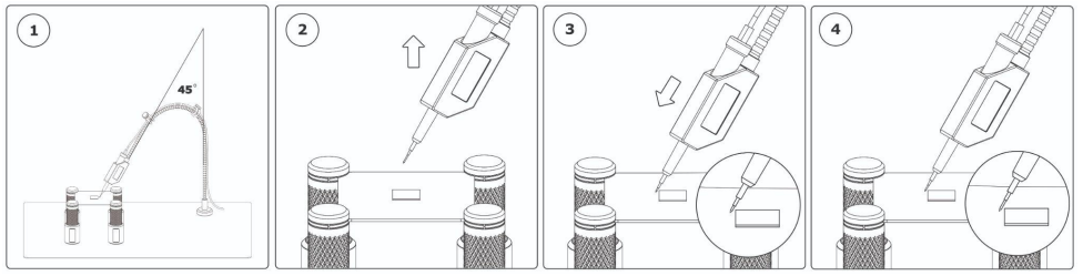
Why must the probe be frequency compensated? ▼
Understanding Probe Compensation
Oscilloscopes inherently have input capacitance, typically in the range of tens of picofarads, which is connected in parallel with the input resistance. While this capacitance doesn’t pose a problem for DC measurements, it becomes critical when measuring AC signals. As frequency increases, the input capacitance starts acting as a low-pass filter, attenuating higher frequencies and distorting the signal.
Probe Compensation and why it is necessary
Probe compensation is the process of adjusting the probe’s capacitance to match and offset the input capacitance of the oscilloscope. Proper compensation ensures accurate, linear measurements across a wide frequency range. Without this adjustment, the probe’s performance can be compromised, leading to inaccurate readings.
When a probe is not properly compensated, two primary issues arise:
Incorrect Amplitudes: A poorly compensated probe can lead to significant variations in signal amplitude, even at lower frequencies. Comparisons between measurements taken with properly and improperly compensated probes show noticeable differences in amplitude, which can impact the accuracy of the results.
Distorted Waveforms: Another consequence of improper compensation is waveform distortion, especially affecting the rise and fall times of pulsed signals. As frequency increases, these distortions become more pronounced, affecting the integrity of high-speed signal measurements.
Timing for Probe Compensation
Probes should always be compensated before first use or when making important measurements. Each oscilloscope has a unique input capacitance, so when a probe is connected to a different oscilloscope, it must be re-compensated to match the new input characteristics. This becomes even more critical at higher frequencies. However, moving the probe between ports on the same oscilloscope generally doesn’t require re-compensation, as the ports usually share the same input capacitance.
How to compensate the probe
Most oscilloscopes include a built-in square wave generator, typically at a frequency of 1 kHz, specifically for probe compensation. The generator is usually labeled "probe compensation" and indicated by a square wave and ground symbol.
1.Connect the probe tip to the square wave output, and the probe ground lead to the ground.
2.Use a non-conductive screwdriver or tool to adjust the compensation capacitor on the probe while observing the square wave signal on the oscilloscope.
3.The goal is to adjust the capacitor until the square wave appears as perfectly rectangular, with horizontal tops and clean edges.
Overcompensated Probe: If the signal shows overshoot on the leading edge of the waveform, the probe is overcompensated.
Undercompensated Probe: If the signal shows undershoot or sagging on the leading edge, the probe is undercompensated.
In both cases, slight adjustments to the probe’s compensation capacitor can correct the waveform. Fine-tuning usually requires just a small fraction of a turn to achieve a properly compensated probe, which results in a crisp, square waveform.
Square waves are ideal for probe compensation because they contain both high and low-frequency components, making them useful for detecting inaccuracies in the probe’s frequency response.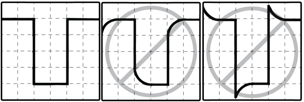
Properly compensated, Undercompensated, Overcompensated
Frequency responce with different compensations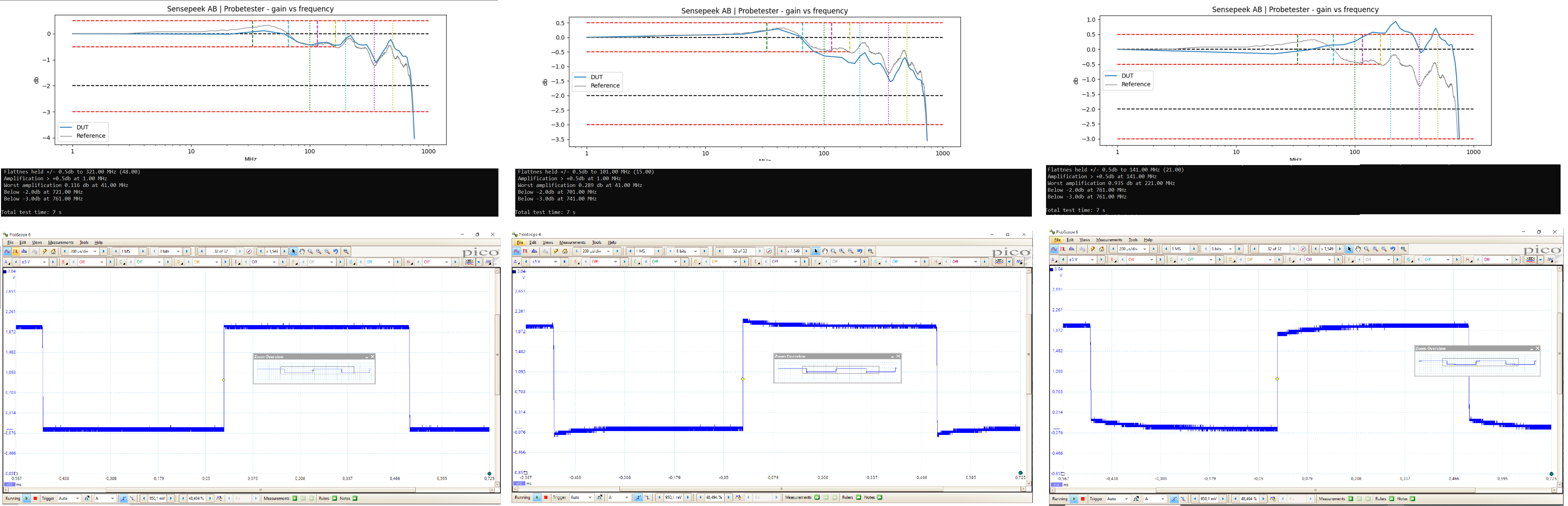
How do I read the Impedance and derating curve in Oscilloscope Probe Datasheets? ▼
When reviewing the datasheet of an oscilloscope probe, understanding its impedance behavior across different frequencies is crucial. A probe rated at 10 MΩ, for instance, typically comprises a 9 MΩ resistor in series with the cable, coupled with a 1 MΩ input impedance from the oscilloscope. This configuration establishes a 10:1 attenuation ratio, meaning that a 10V test signal is reduced to 1V at the oscilloscope’s input.
However, the datasheet indicates that the impedance decreases as frequency increases, which is a natural phenomenon but critical for users to recognize. This characteristic implies that the probe will increasingly load the circuit under test at higher frequencies, potentially impacting measurement accuracy and circuit performance. Understanding this behavior is essential for selecting the appropriate probe and ensuring accurate measurements in high-frequency applications.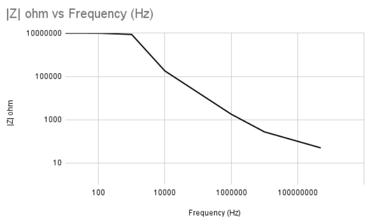
Impedance vs frequency curve for a 10:1 probe
Voltage Derating
Another often-overlooked aspect in the oscilloscope probe datasheet is the voltage derating curve over frequency. A common question arises: why can’t the probe measure high voltage at high frequencies? The answer lies in both the electrical and mechanical properties of the probe itself.
The probe cable functions as a large mechanical capacitor. As the frequency of the input signal increases, the capacitive coupling between the inner conductor and the outer plastic sheath, typically handled by the user, intensifies. This increased coupling can lead to unwanted effects, especially regarding safety. According to oscilloscope probe safety standards set for 2024, the maximum allowable current must not exceed 70 mA to protect the user from electrical hazards. Consequently, this current limitation results in a voltage cap of 35V for frequencies approximately above 5 MHz.
At these higher frequencies, certain components within the probe’s frequency compensation circuitry are subjected to greater stress. If these components are overloaded, there is a risk of failure, which could compromise the probe’s performance and the safety of the user. This relationship is illustrated in the derating curve presented in the datasheet, which combines the capacitive effects of the probe cable with the operational limits of its internal components.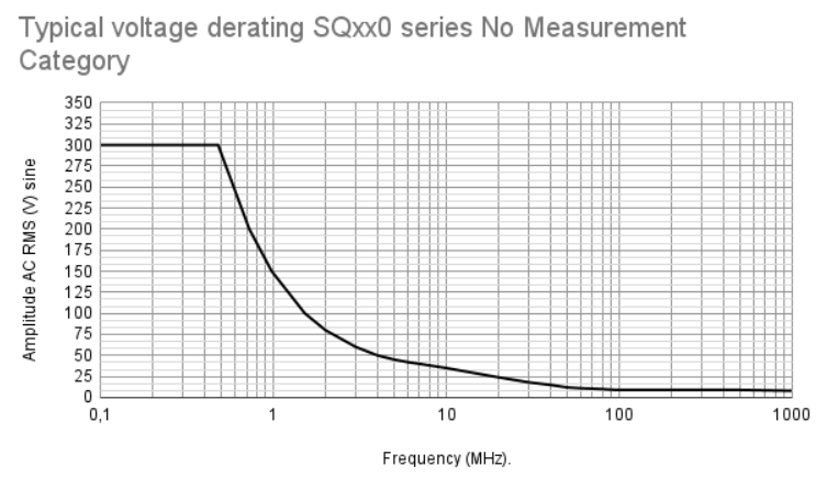
Voltage derating curve for a 10:1 probe
FAQ REPLACE
I have bent / broken my needle tip on my probe, what should I do? ▼
Here are new signal needles, if you have a SP10 probe and the needle is stuck inside you can change the holder by simply solder in a new one.
ProbeTipNeedle
NeedleHolder
How do I change the signal needle? ▼
Probe needle replacement
1. Notice the replaceable needle tip. Please be aware of the sharp needle tip!
2. Pull out the replaceable needle tip by hand or use pliers.
3. Pick up the new needle tip and insert in the sleeve with pliers.
4. Press the needle vertically against a planar stable surface and make sure it is correctly inserted.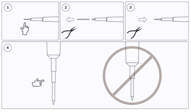
Replacing signal needle on SQ-xx0 series ▼
Yes, follow the guide here
Replacing signal needle on SQ-xx0 series