100 MHz
PCBITE-6013
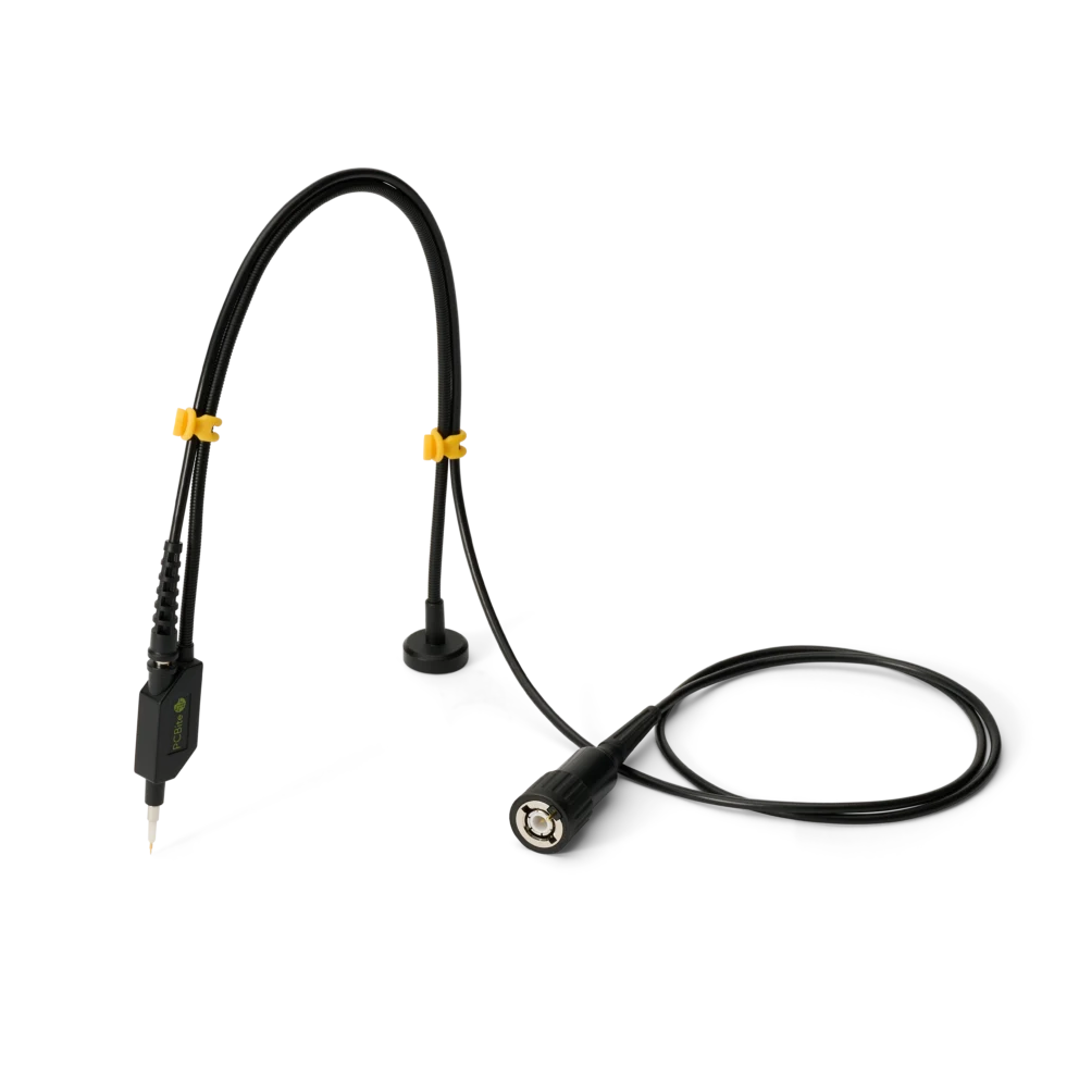
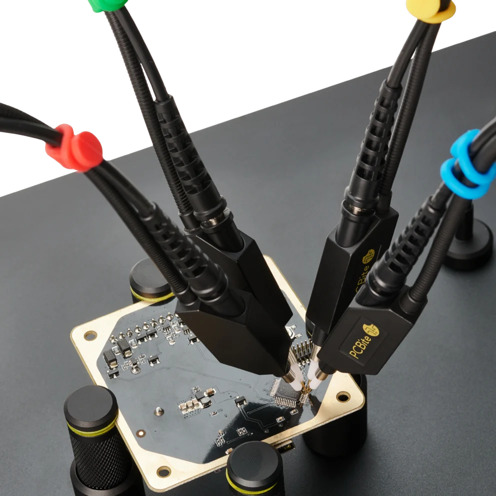
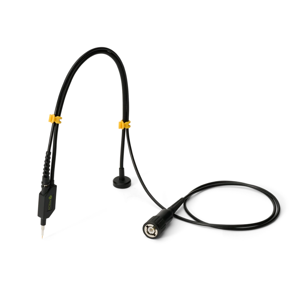
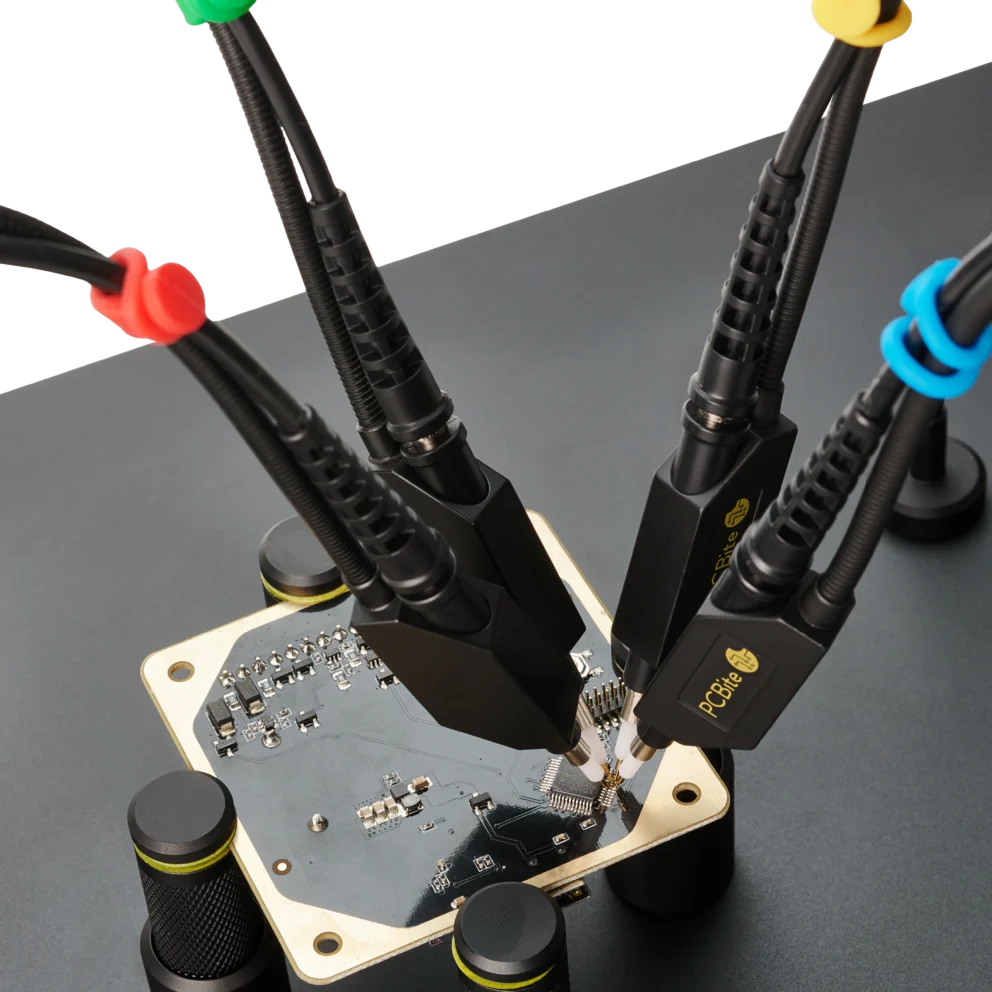
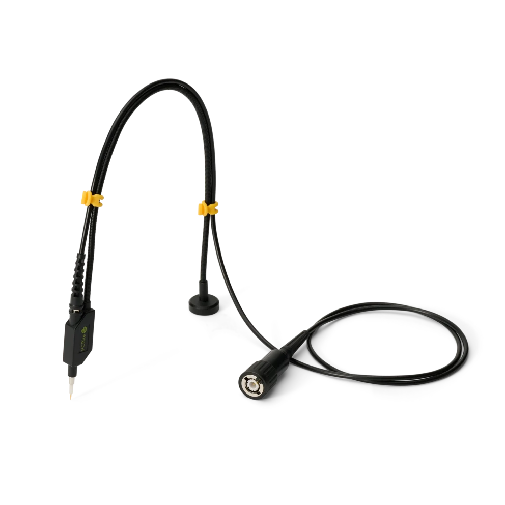
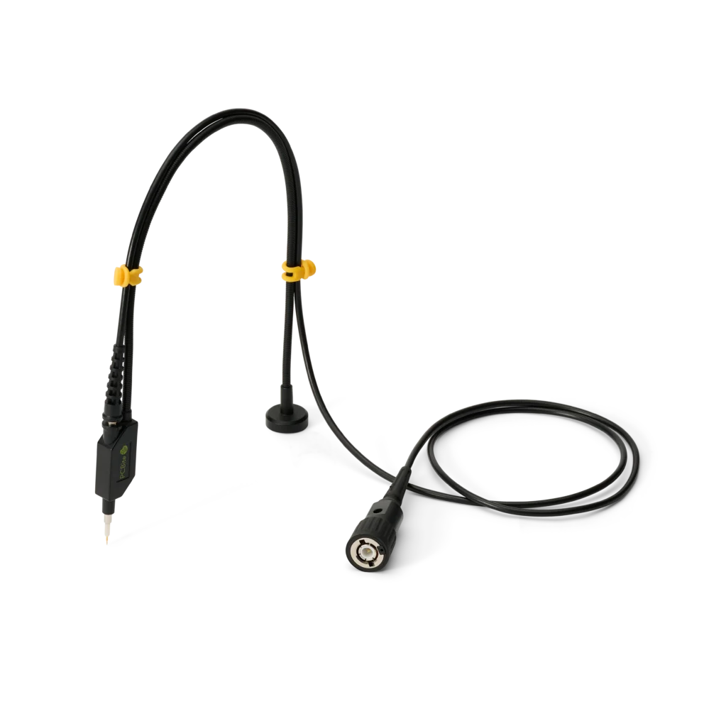
SQ100 – 100 MHz handsfree oscilloscope probe
59 €
In stock
A common question is whether a 93 MHz clock can be measured with a 100 MHz oscilloscope and a 100 MHz probe. It seems reasonable, but together they have a bandwidth of about 71 MHz, so the clock is shown too small and rounded. This article explains why, and how to choose a probe that lets your oscilloscope show what it can.
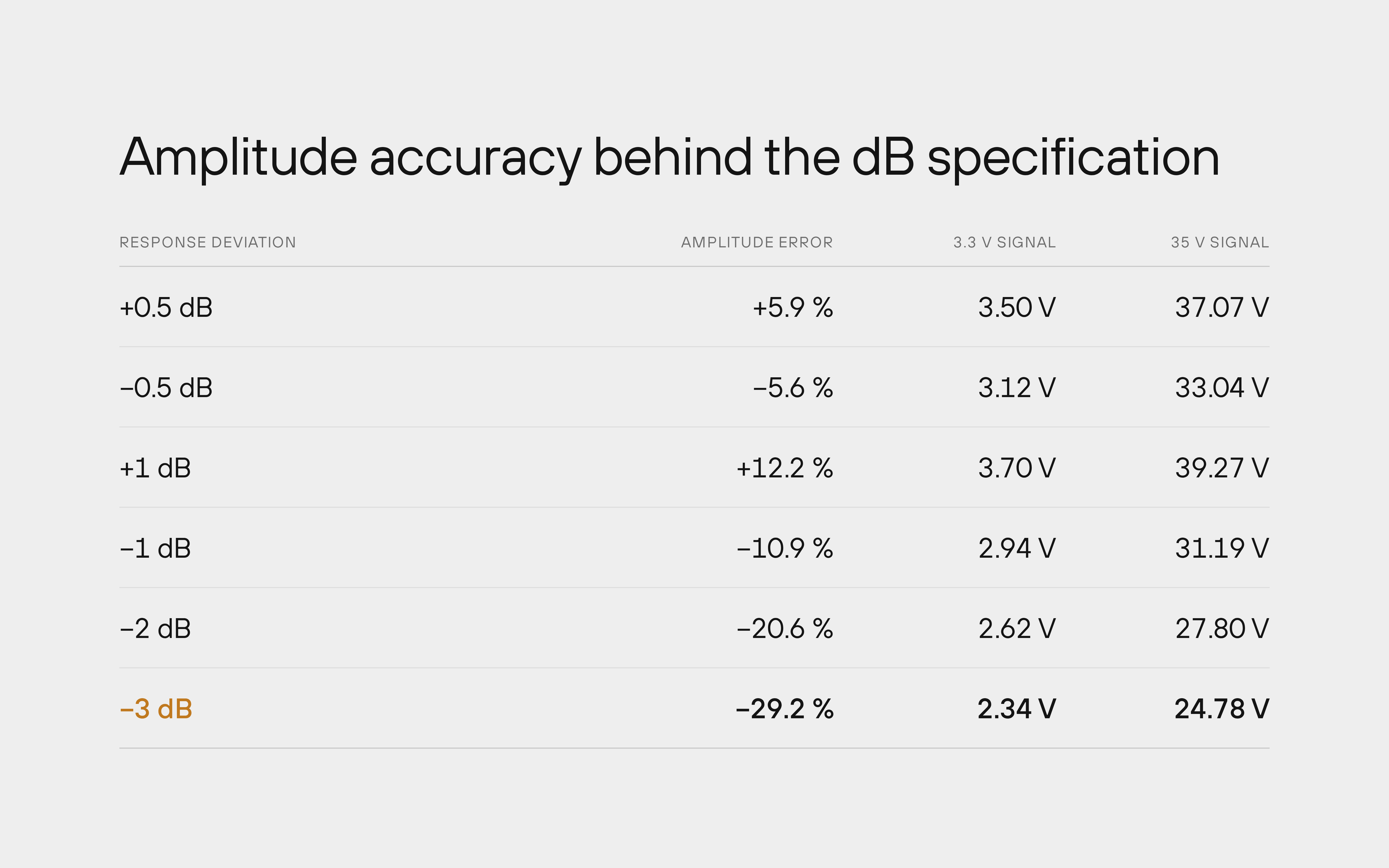
Bandwidth is the frequency at which a sine wave is shown 3 dB lower than at low frequencies, at about 70.7 % of its true amplitude (IEEE 1057). Oscilloscopes and probes are both specified this way.
At its bandwidth limit, an instrument already shows almost 30 % too little.
The oscilloscope and the probe each have their own bandwidth, but the signal passes through both, and the losses add up. Manufacturers rarely talk about the combination, the system bandwidth.
Most oscilloscopes up to a few hundred MHz have a Gaussian response, which rolls off gradually. For them, the system bandwidth is:
System bandwidth = 1 / √(1/oscilloscope bandwidth² + 1/probe bandwidth²)
The result is always lower than the lower of the two. When both have the same bandwidth, the system reaches about 71 % of it.
| Oscilloscope | Probe | System bandwidth |
|---|---|---|
| 100 MHz | 100 MHz | about 71 MHz |
| 100 MHz | 200 MHz | about 89 MHz |
| 100 MHz | 350 MHz | about 96 MHz |
| 100 MHz | 500 MHz | about 98 MHz |
| 200 MHz | 200 MHz | about 141 MHz |
| 200 MHz | 350 MHz | about 174 MHz |
| 200 MHz | 500 MHz | about 186 MHz |
| 350 MHz | 350 MHz | about 247 MHz |
| 350 MHz | 500 MHz | about 287 MHz |
System bandwidth with a Gaussian oscilloscope response.
Back to the 93 MHz clock. With a 100 MHz probe on a 100 MHz oscilloscope, the clock lies well above the system bandwidth of about 71 MHz: its amplitude is shown too low, and the edges are gone.
A 350 MHz probe on the same oscilloscope raises the system bandwidth to about 96 MHz, close to what the oscilloscope can do on its own. To see the square edges of a clock, the system needs several times the clock frequency, about five times as a rule of thumb.
Some oscilloscopes, mostly at higher bandwidths, have a brickwall response: flat almost up to the bandwidth, then a sharp cutoff. It keeps amplitudes accurate below the cutoff, and suppresses noise and aliasing above it.
With a brickwall oscilloscope, the system bandwidth is close to the lower of the two bandwidths. A 200 MHz brickwall oscilloscope with a 350 MHz probe gives about 200 MHz, where a Gaussian one gives about 174 MHz.
The oscilloscope’s datasheet usually gives its rise time. Multiply the rise time by the bandwidth: about 0.35 means a Gaussian response, 0.4 to 0.45 a brickwall response.
For example, a 350 MHz oscilloscope with a rise time of 1 ns gives 350 MHz × 1 ns = 0.35, so it has a Gaussian response.
Many oscilloscopes and probes have some margin above their rated bandwidth, so a measurement can come out a little better than the formula. The formula is still the right way to compare.
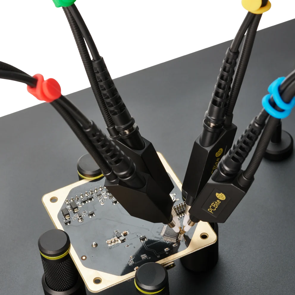
The PCBite oscilloscope probes cover 100 to 500 MHz with the SQ100, SQ200, SQ350 and SQ500, and the SQG series reaches 1.5, 3 and 6 GHz on instruments with a 50 Ω input.
Du använder en föråldrad webbläsare. Alla funktioner fungerar inte i din webbläsare. Var vänlig uppgradera din webbläsare för att förbättra din upplevelse och öka din säkerhet.