1.5 GHz AC
PCBITE-7008
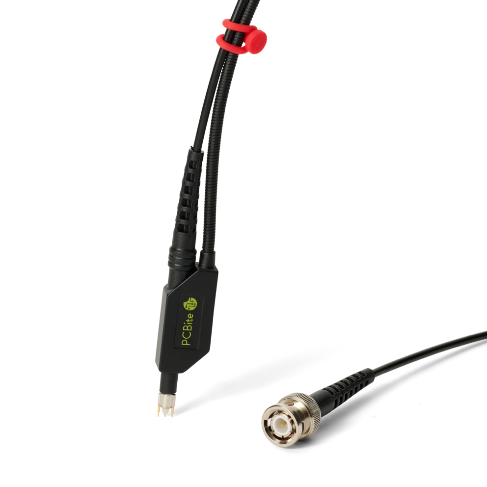
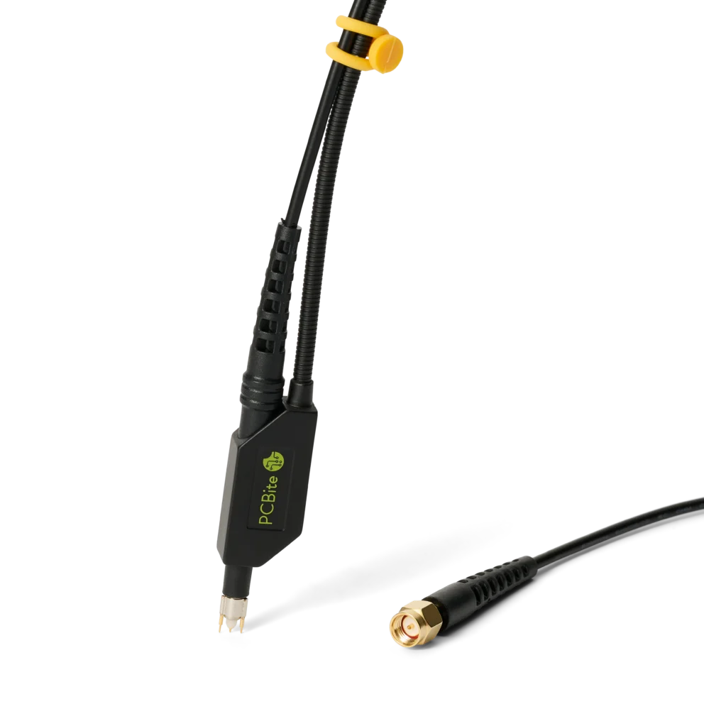
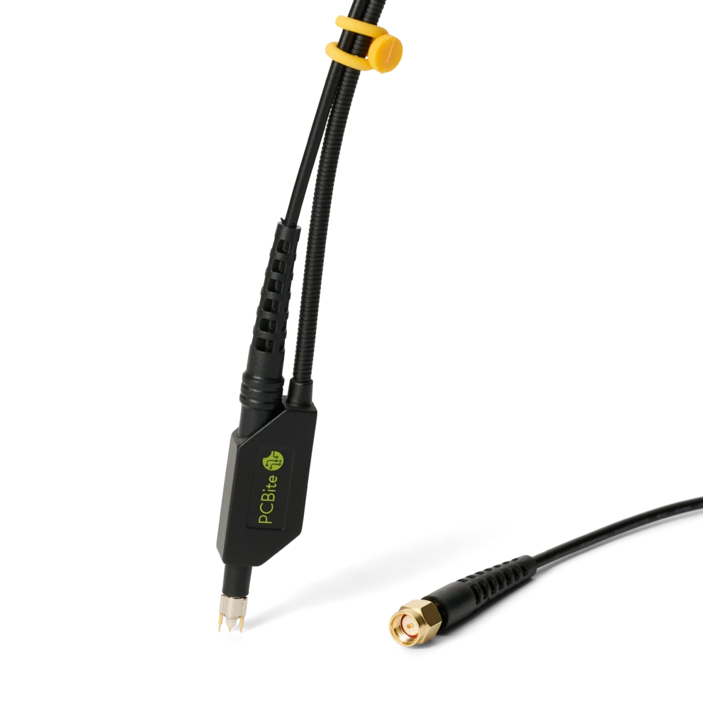
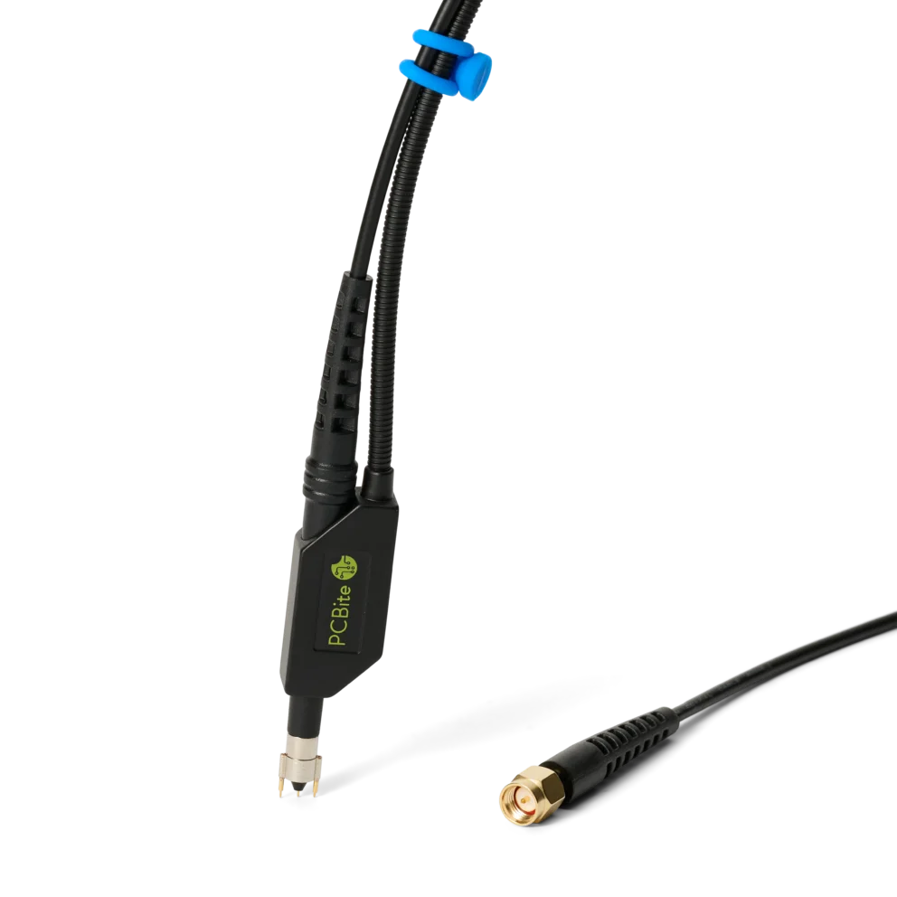
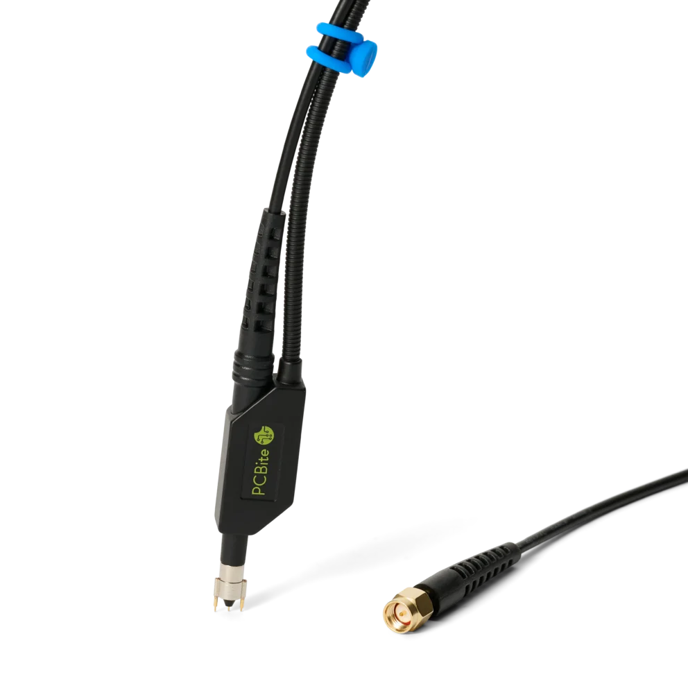
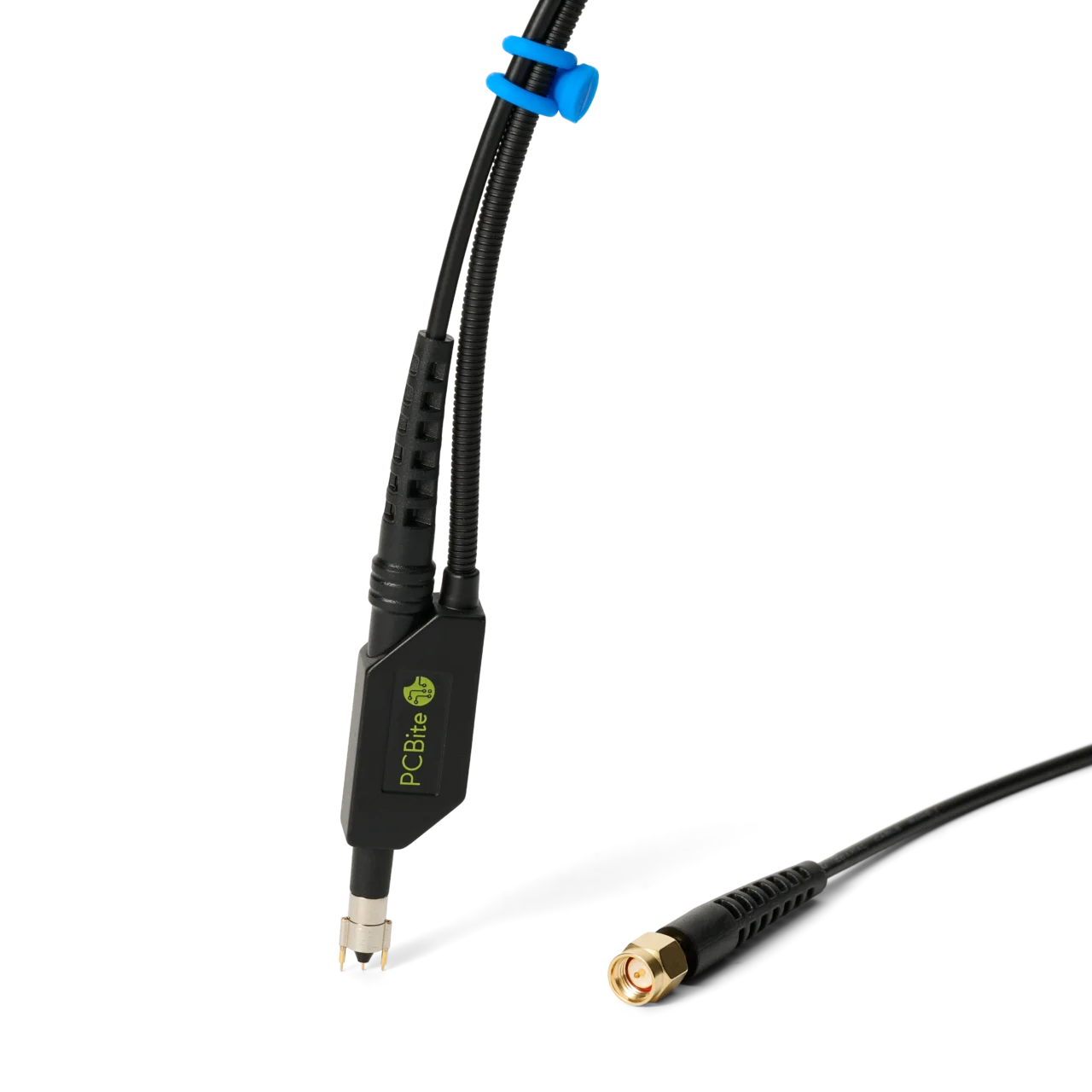
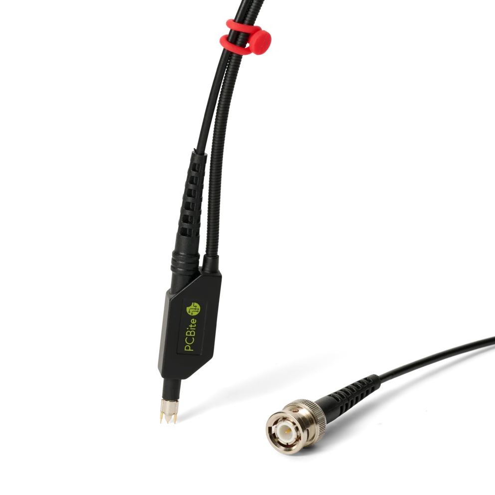
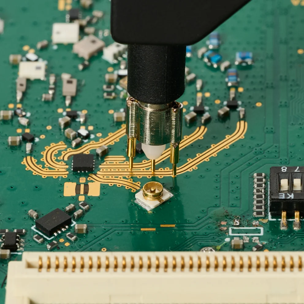
SQG15-AC – 1.5 GHz low impedance 10:1 passive AC probe
169 €
In stock
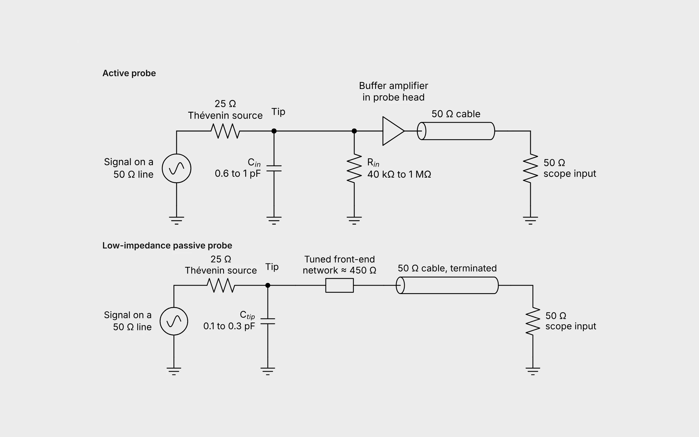
Fig. 1. Simplified models of an active and a low-impedance passive probe on a 50 Ω line.
Active probes have a buffer amplifier in the probe head. Low-impedance passive probes, also called Z0, 50 Ω or voltage divider probes, have none1. This article explains why the passive type is a strong alternative for GHz work, and when it can outperform an active probe.
Any probe adds a resistance in parallel with a capacitance from the probed node to ground. As the frequency increases the capacitive reactance falls and takes over1, 2.
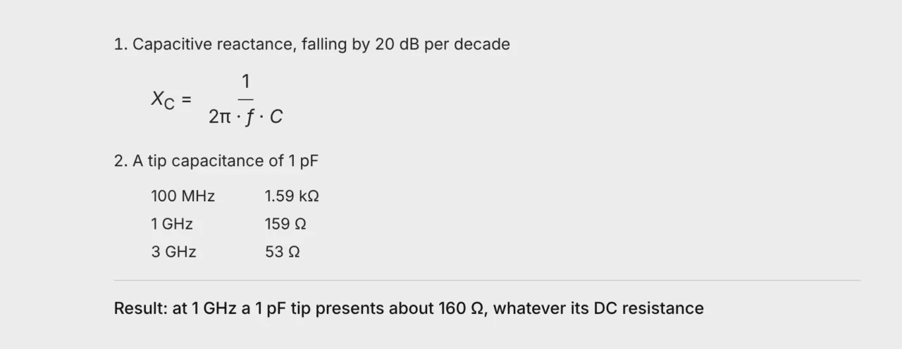
Measured active probes can dip even lower in the upper part of their bandwidth, to between 15 Ω and a few hundred ohms3, 4, 5.
The tip feeds a 50 Ω cable terminated by the 50 Ω instrument input. A terminated cable hides its own capacitance, so the circuit sees only the tip network in series with 50 Ω1, 6.
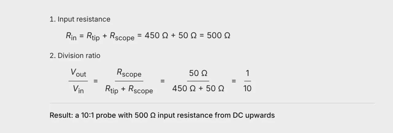
On paper the tip is a single 450 Ω resistor. In a real GHz probe it is a network of components that together behave as 450 Ω. The needle, mechanics, PCB layout and cable transition are tuned together so that the network stays resistive and the response stays flat into the GHz range.
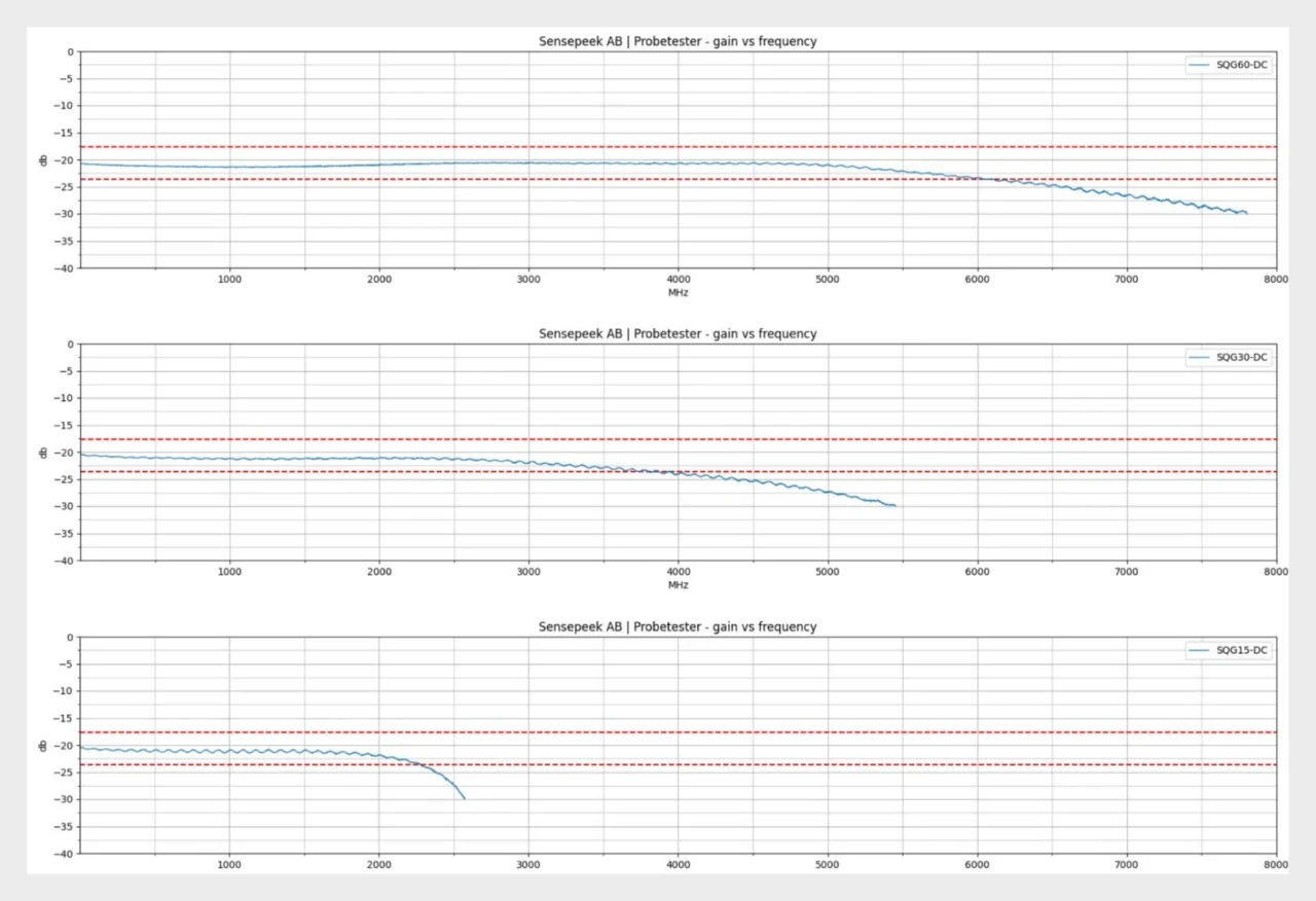
Fig. 2. Measured gain versus frequency of production SQG60-DC, SQG30-DC and SQG15-DC probes. The level of about −20 dB is the 10:1 division ratio. The response is flat within ±0.5 dB from DC to 5.2 GHz, 2.7 GHz and 1.5 GHz respectively7.
A flat response divides every frequency component by the same factor. Edges, ringing and harmonics reach the instrument in the right proportions.
Figure 3 compares the modelled impedance of the two probe types. Below roughly 370 MHz the active probe loads the circuit less. Above it a 500 Ω probe with low tip capacitance presents the higher impedance and outperforms the active probe. At GHz frequencies the tip capacitance decides, not the DC resistance.
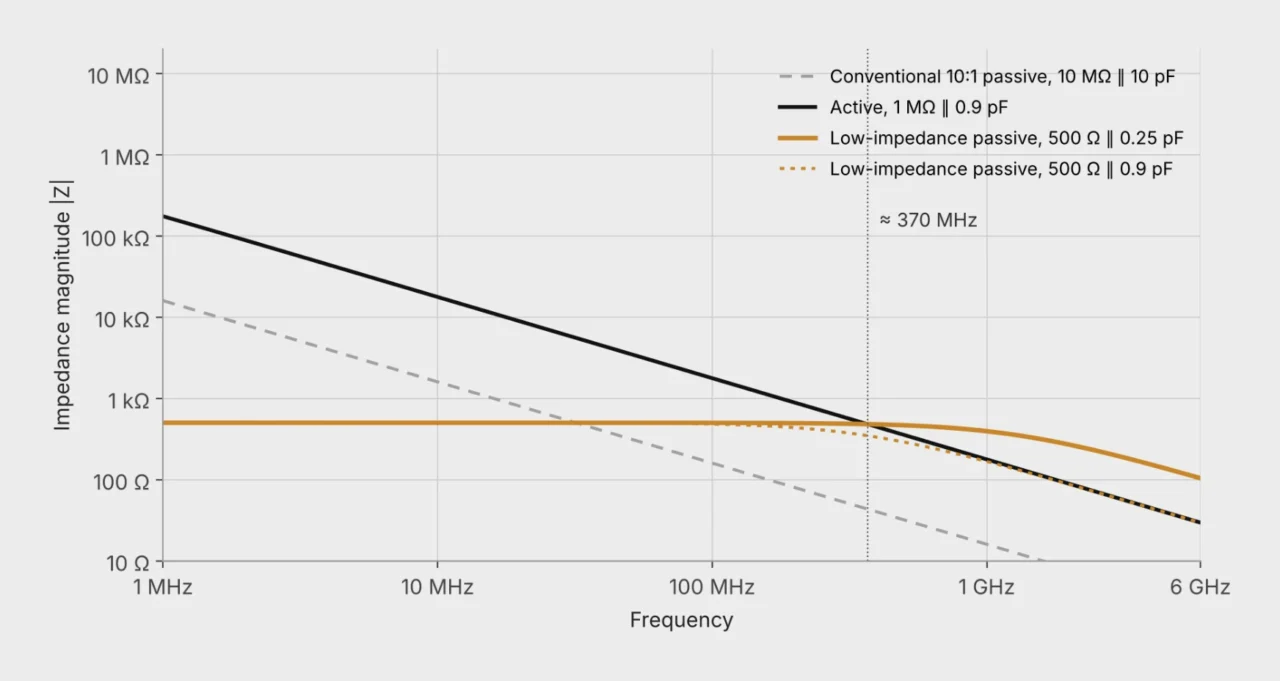
Fig. 3. Modelled input impedance of a conventional 10:1 passive probe, an active probe and generic low-impedance passive probes with two values of tip capacitance. Calculated as |Z| = |R ∥ 1/(j2πfC)|. The curves illustrate the principle and do not represent a specific product.
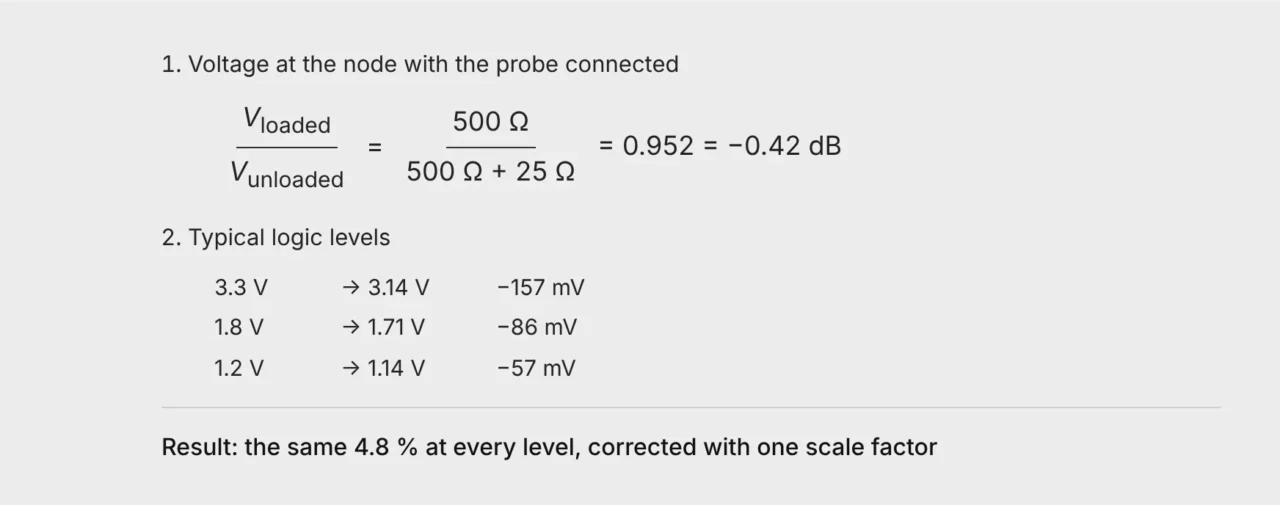
On a 50 Ω line the 500 Ω is a light load. A point on a line terminated at both ends behaves like a 25 Ω source2, 5, so the probe leaves 500/525 of the voltage, or −0.42 dB.
Wide signal range. Typical 1.5 GHz to 3.5 GHz active probes have a linear range of ±8 V, some only ±4 V8, 9, 10, 11. A passive divider has no amplifier that can saturate. Its limit is the voltage and power rating of the front end.
Robustness. Active probes can be damaged by electrostatic discharge1, 12. Passive probes are more robust to overvoltage and ESD6.
Any 50 Ω instrument. An active probe needs power and the manufacturer’s probe interface12. A passive probe works with any oscilloscope, sampling oscilloscope, network analyzer or spectrum analyzer with a 50 Ω input.
Low added noise. A 10:1 probe raises the instrument noise, referred to the tip, by a factor of ten. Most active probes in this class also divide by ten8, 9 and add 1.2 mV to 2.5 mV RMS of amplifier noise on top8, 11. A passive divider adds only a few microvolts of thermal noise.
Cost. Distributor prices for 1.5 GHz to 3.5 GHz active probes, checked in October 2026, ranged from about USD 3,000 to USD 8,00013. Low-impedance passive probes for 1.5 GHz to 6 GHz are available from about USD 190 to USD 3907, so an AC-coupled and a DC-coupled probe can both be on the bench for a fraction of the price of one active probe.
A DC-coupled probe shows the complete signal including logic levels and bias. Its 500 Ω also loads the DC level, which is fine on low-impedance outputs, terminated lines and supply rails. An AC-coupled probe adds a DC block, so no DC current flows through the probe. Use it on DC-biased high-speed links such as USB, PCIe, SATA and HDMI, and for ripple on supply rails7.
A 500 Ω probe is not meant for high-impedance nodes. On an I²C line with a 10 kΩ pull-up to 5 V it would pull the idle level down to about 0.24 V14. Such measurements are best made with a high-quality conventional 10:1 passive probe, such as the PCBite SQ100 to SQ500. Its 10 MΩ leaves the bias undisturbed, and its tip capacitance of around 10 pF is small next to the 400 pF the I²C specification allows per bus line15.
Active probes fill the gap between the two passive types, with fast signals on high-impedance nodes and instruments that have only 1 MΩ inputs14.
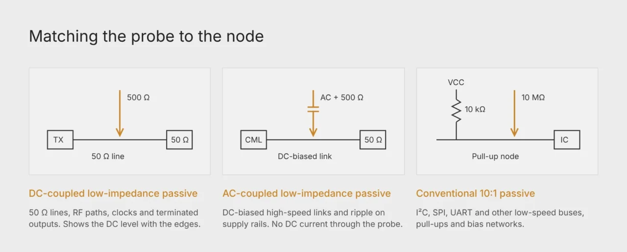
Fig. 4. The impedance, DC level and speed of the node decide which probe disturbs the circuit least.
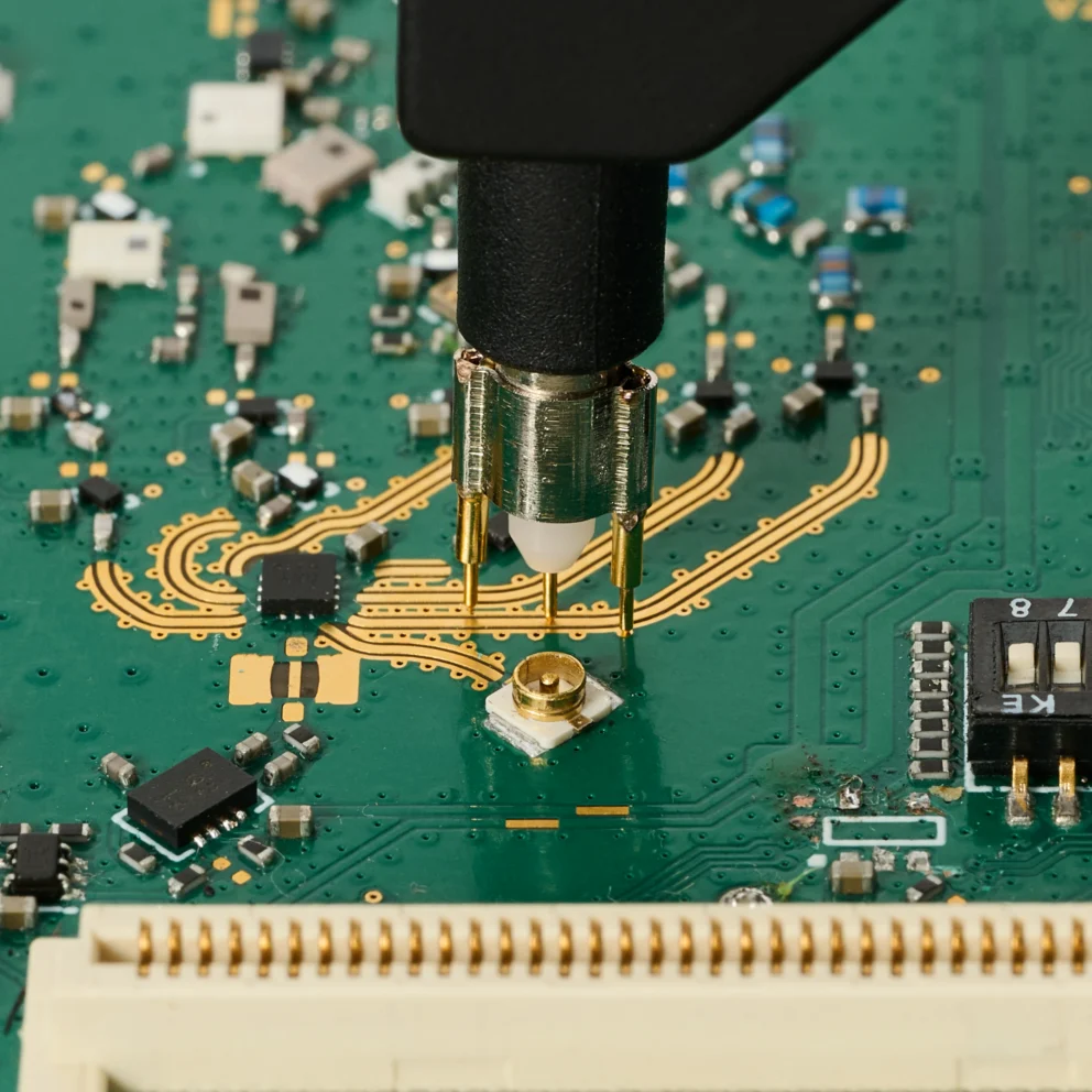
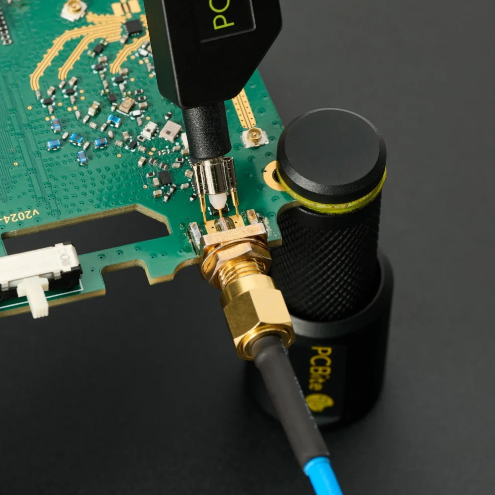
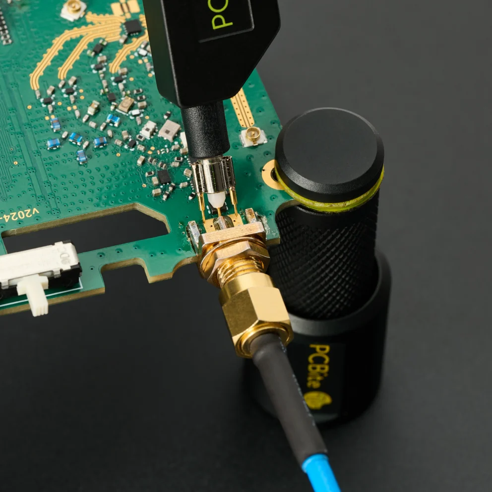
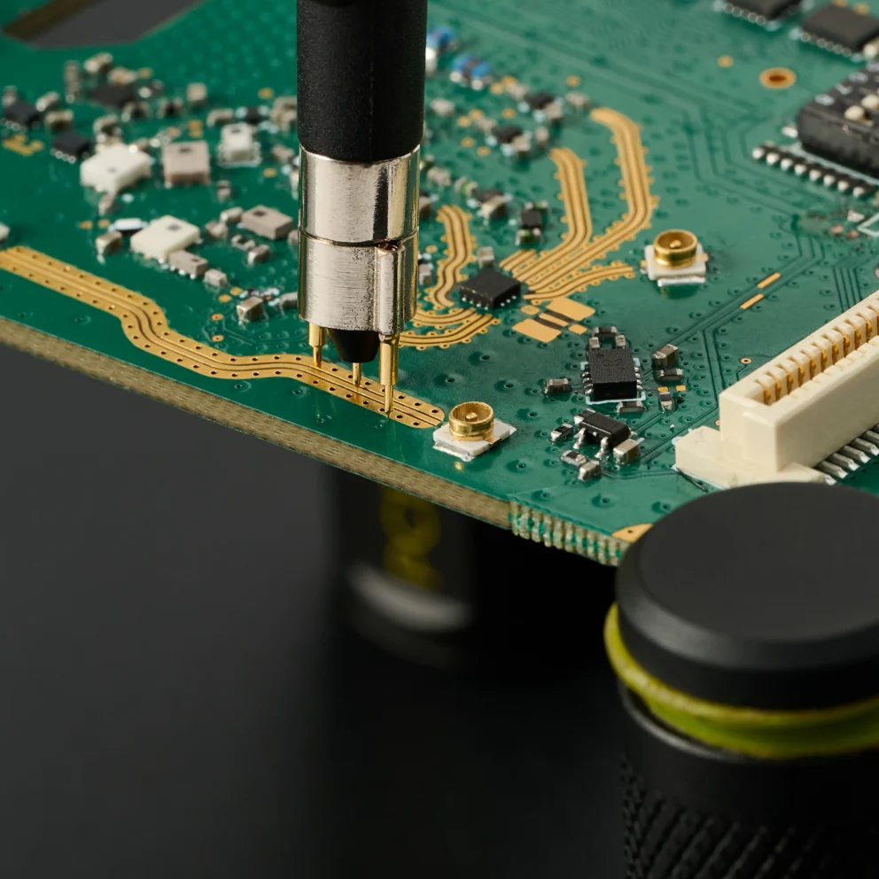
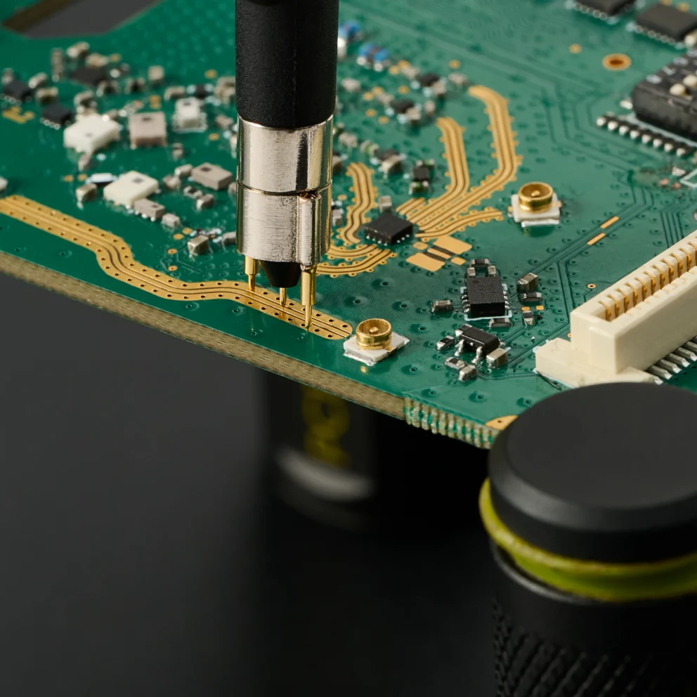
The PCBite SQG series offers handsfree low-impedance probes for 1.5 GHz, 3 GHz and 6 GHz, each in AC-coupled and DC-coupled versions7.
See the SQG high-frequency probes.
Du använder en föråldrad webbläsare. Alla funktioner fungerar inte i din webbläsare. Var vänlig uppgradera din webbläsare för att förbättra din upplevelse och öka din säkerhet.