100 MHz
PCBITE-6013
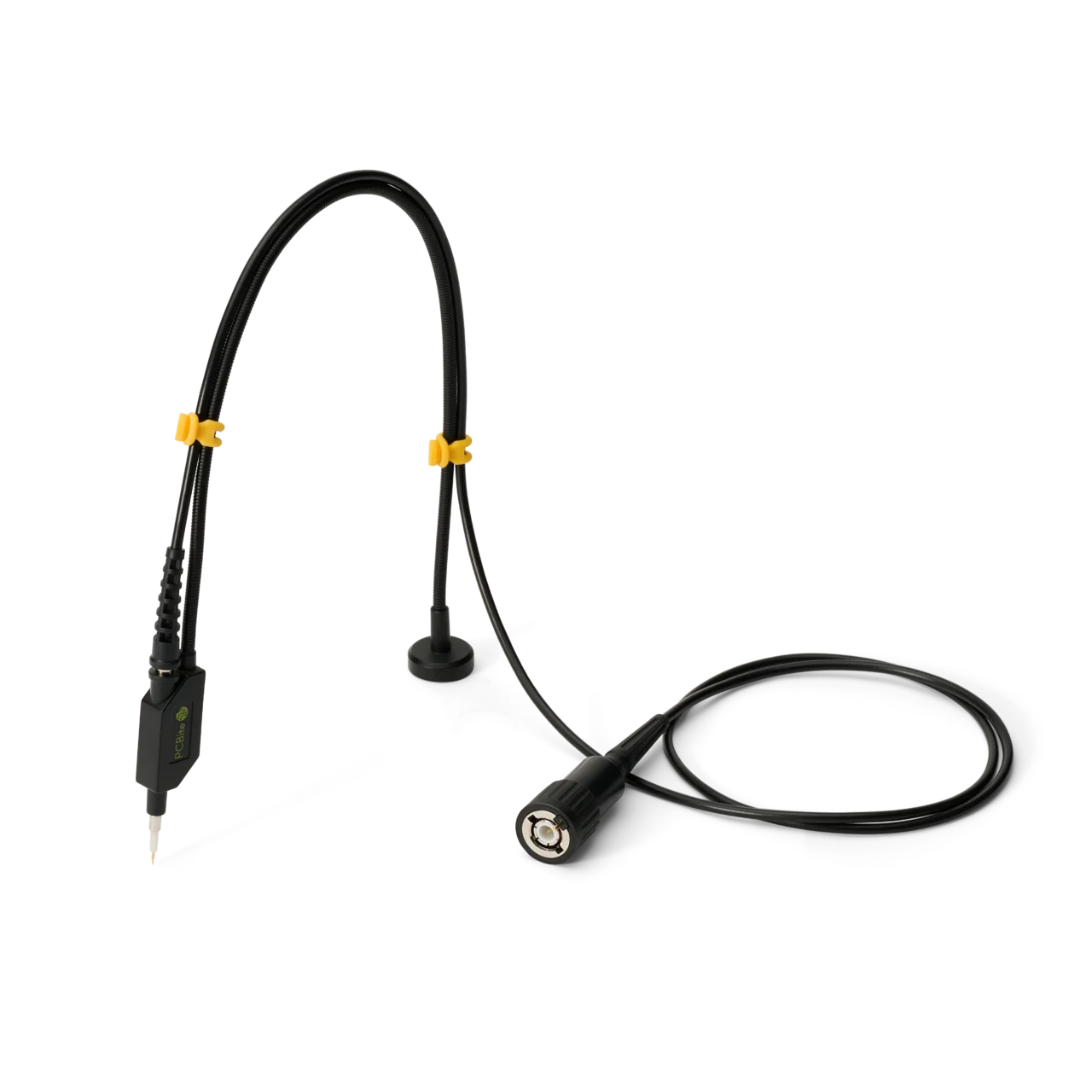
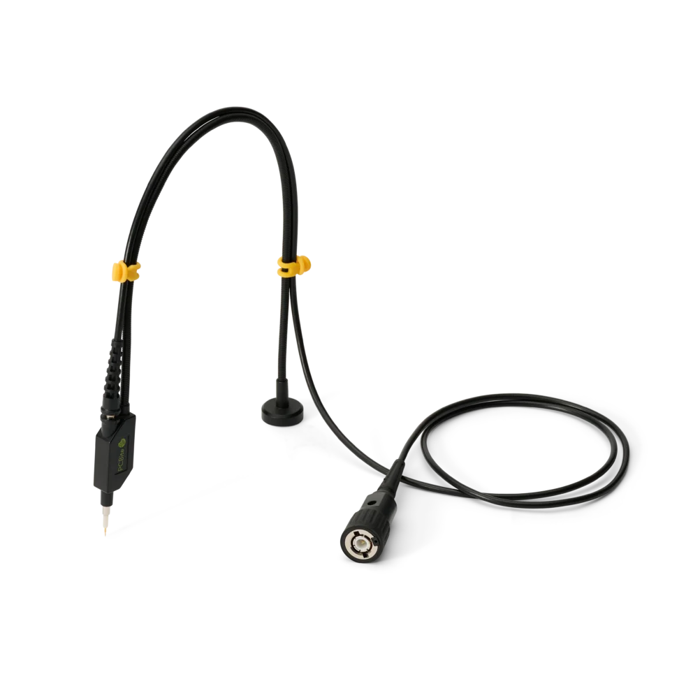
SQ100 – 100 MHz handsfree oscilloscope probe
59 €
In stock
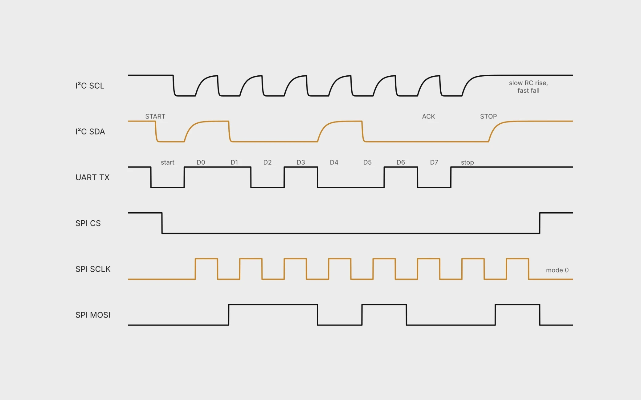
Fig. 1. Typical waveforms. I²C with open-drain edges, a UART frame with start bit, eight data bits sent LSB first and a stop bit, and an SPI transfer in mode 0.
I²C uses two lines, SDA and SCL. Every device has an open-drain output that can only pull the line low. Pull-up resistors to the supply create the high level, so the bus forms a wired-AND1. The three open-drain modes run at up to 100 kbit/s in Standard-mode, 400 kbit/s in Fast-mode and 1 Mbit/s in Fast-mode Plus. The specification also defines a High-speed mode at 3.4 Mbit/s and a push-pull Ultra Fast-mode at 5 Mbit/s, which are not covered here. Data on SDA must be stable while SCL is high. A falling SDA edge while SCL is high is a START, a rising edge is a STOP1. The falling edges are driven, but the rising edges are set by the pull-up resistor and the bus capacitance, and every probe adds capacitance to the bus.
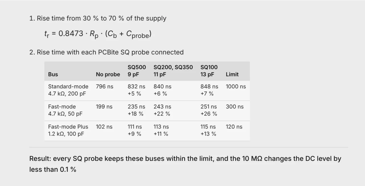
The I²C specification limits the rise time to 1000 ns in Standard-mode, 300 ns in Fast-mode and 120 ns in Fast-mode Plus1, 2. With every SQ probe these buses stay within their rise time limits, even though the probe slows the edge by up to about a quarter on a lightly loaded bus. The oscilloscope shows the bus with the probe connected, so the real edge is slightly faster than the one on the screen. On a bus that is already close to its limit, choose the probe with the lowest tip capacitance.
UART is asynchronous. Each direction has its own line that idles high. A frame starts with a low start bit, followed by five to nine data bits sent LSB first, an optional parity bit and one or two high stop bits3. There is no clock line, so both ends must agree on the baud rate. The baud rate is simply the number of bits sent per second, start and stop bits included. At 115 200 Bd each bit lasts 1/115 200 s = 8.68 µs, and a ten-bit frame carries one byte in 86.8 µs.
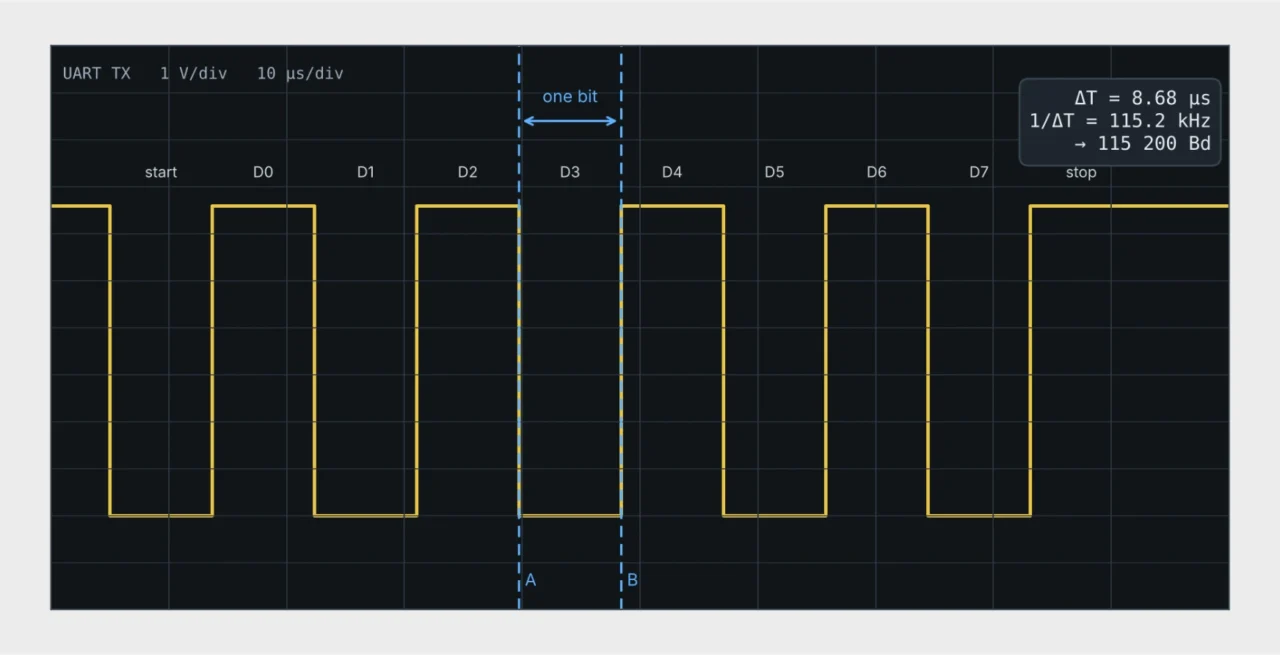
Fig. 2. Measuring the baud rate. Send 0x55, which alternates ones and zeros, place the cursors on the edges of one bit and read 1/ΔT. Here ΔT = 8.68 µs gives 115 200 Bd.
The receiver samples each bit near its center. With the common 16× oversampling and a ten-bit frame, the clocks at the two ends may differ by about ±3.3 % in total when each bit can be sampled cleanly over about three quarters of its width, and by only about ±2 % when slow or distorted edges leave just the middle half4. Compare the measured bit time with the nominal value. UART pins on a microcontroller use logic levels. An RS-232 port uses inverted levels between ±3 V and ±15 V at the receiver5, so check the instrument input range before connecting.
SPI is synchronous and full duplex, with a clock SCLK, data lines MOSI and MISO and an active-low chip select CS. Four modes set the clock polarity and the edge that samples the data6. SPI has no formal standard, uses push-pull outputs and often runs above 10 MHz7. Fast push-pull edges on long traces are where overshoot and ringing appear.
Timing is a digital question. Is the clock frequency right, do START, STOP, ACK and chip select come where they should, does the SPI mode match on both sides, and is the I²C data setup time met (250 ns in Standard-mode, 100 ns in Fast-mode)1? A logic analyzer answers this over long captures and decodes the bytes.
Signal quality is an analog question. Is the low level below 0.3 of the supply and the high level above 0.7 of the supply, as I²C requires1? Are rise times within the specification? Is there overshoot, undershoot or ringing? One reason to measure overshoot and undershoot is to make sure the input protection never starts to conduct. Inputs are protected in different ways, so the absolute maximum ratings in the device data sheet set the limit. Standard logic with clamp diodes is typically rated to 0.5 V beyond the supply rails8, while STM32 3.3 V pins allow 0.3 V below ground and 0.3 V above VDD9. If the limit is not known, keeping the signal within 0.3 V of the supply rails is a conservative rule of thumb. Slow edges that linger near the threshold can make an input switch more than once10. Only an oscilloscope shows these effects.
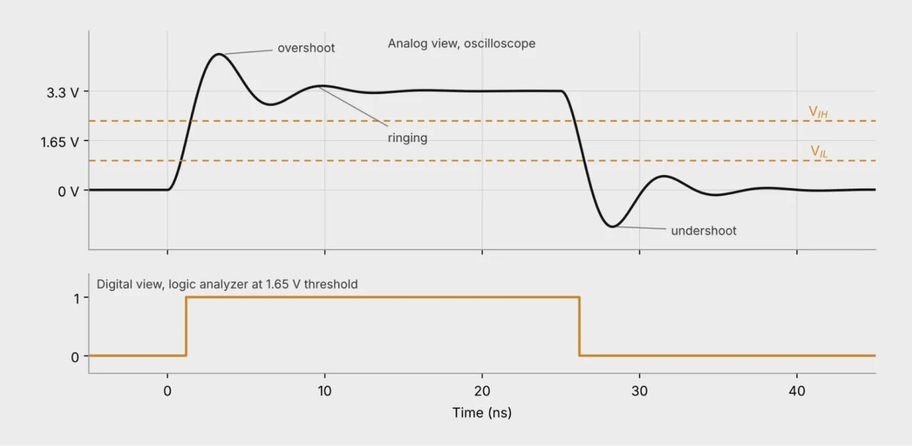
Fig. 3. The same 3.3 V edge seen by an oscilloscope and by a logic analyzer. The logic analyzer shows a clean transition, while the oscilloscope shows overshoot, ringing and undershoot below ground. Illustration.
A 10:1 passive oscilloscope probe has an input resistance of 10 MΩ and a capacitance around 10 pF11. The high resistance leaves pull-ups and bias points undisturbed. The bandwidth decides how fast an edge the probe can show, and that depends on how the edge is defined. There is no common definition across the three buses.
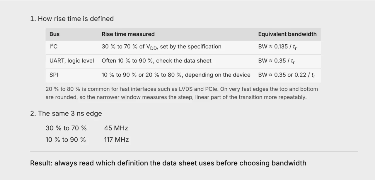
The factors assume a simple RC edge. 0.35 / BW is the standard relation for 10 % to 90 %11, 12.
The probe and the oscilloscope add their own rise time to the signal. The measured value is approximately the square root of the sum of their squares12. A system three times faster than the edge measures it within 5 %, five times faster within 2 %11.
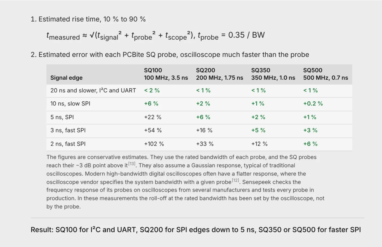
Our article on system bandwidth explains how probe and oscilloscope combine.
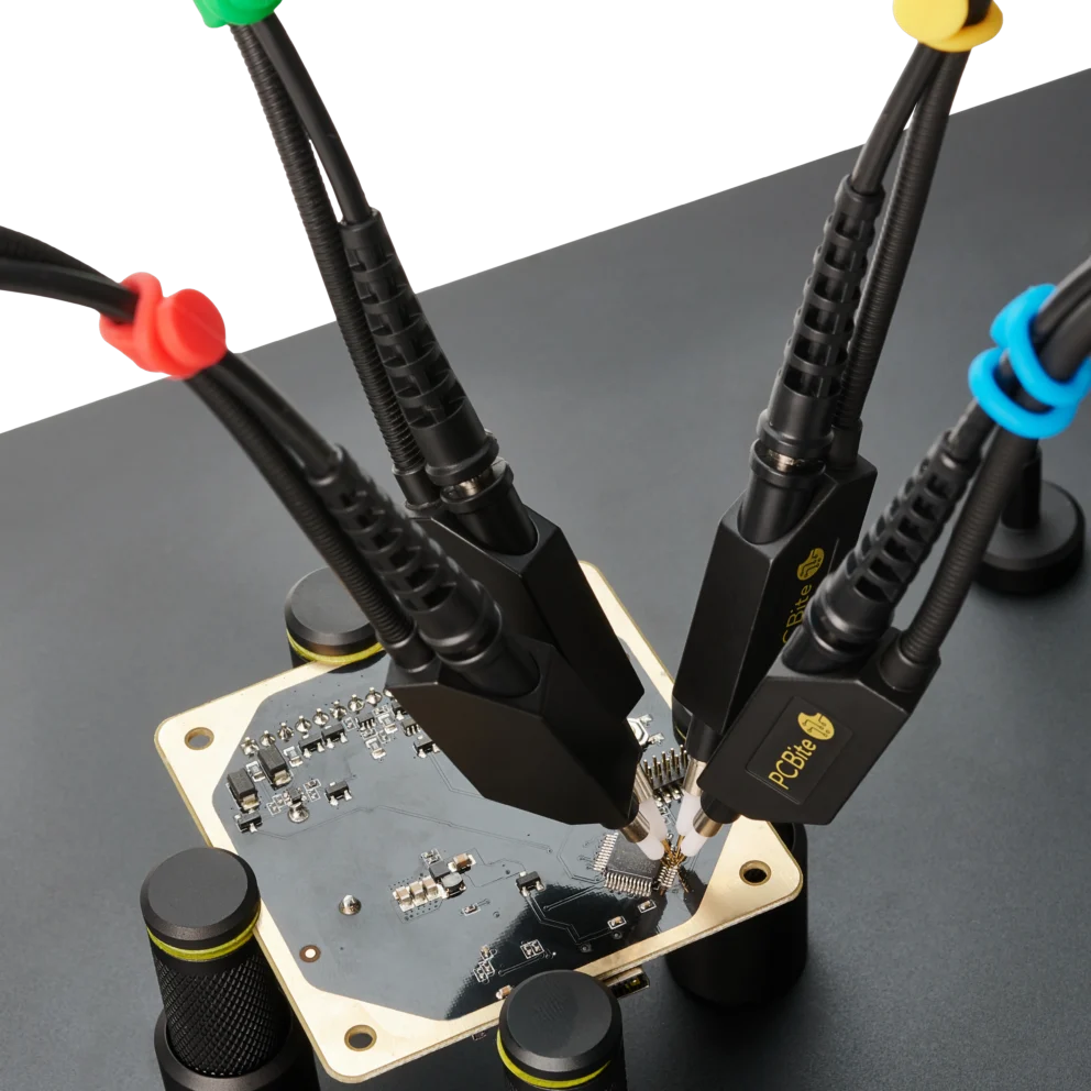
The ground connection matters as much as the bandwidth. A ground lead adds inductance and a loop that picks up noise11, 13. A long ground lead and the probe capacitance form a resonant circuit. In Sensepeek’s tests with the 170 mm (6.7 in) alligator ground cable the gain rises sharply above about 15 MHz, which shows up as false overshoot and ringing on fast edges. Use the long lead to find the signal or to measure signals below about 15 MHz, and switch to the ground spring needle for edges and faster signals. The SQ probes are tuned for a flat frequency response with it and reach their full rated bandwidth in handsfree use13. Where external noise must be kept out, the MMCX adapter gives the shortest ground path and the smallest loop.
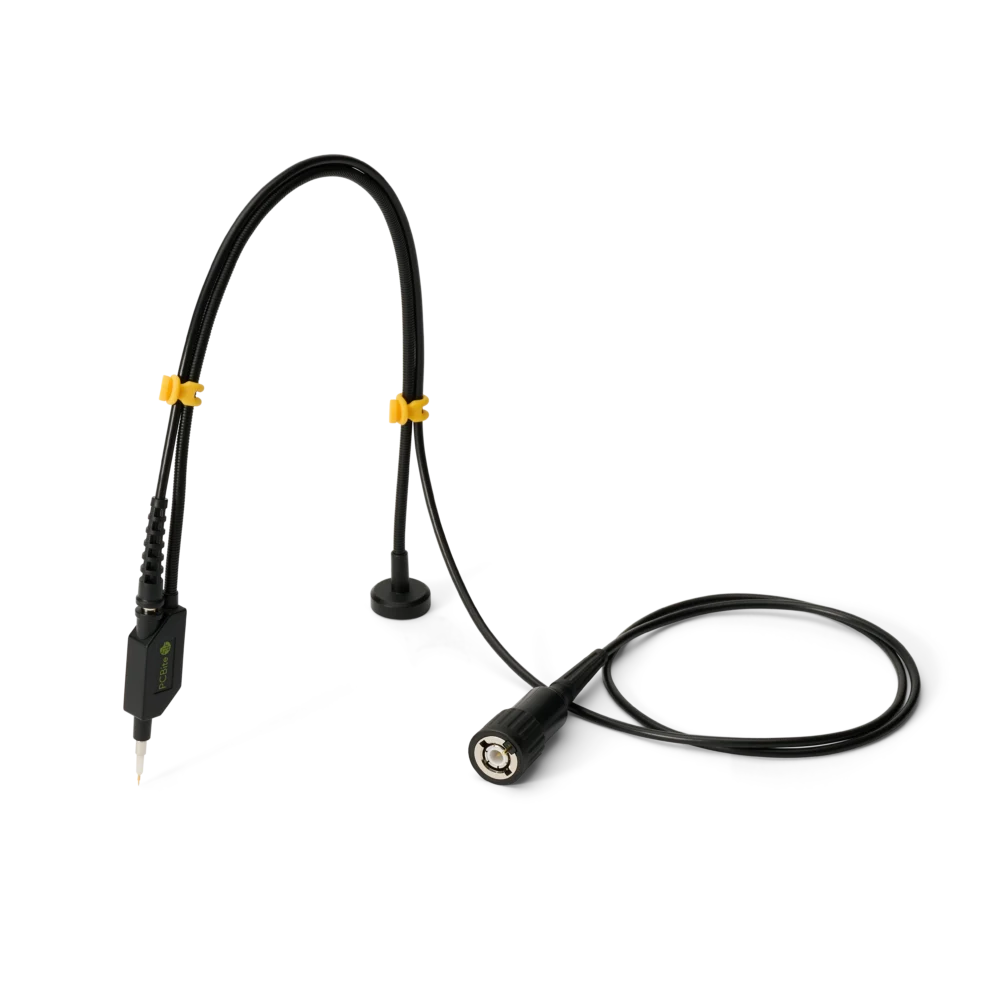
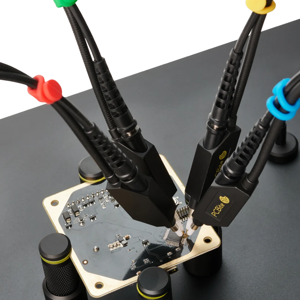
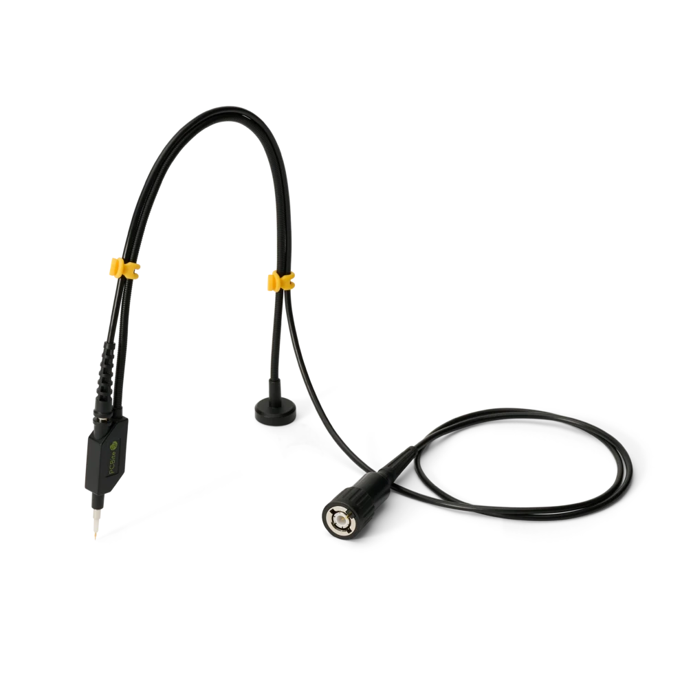
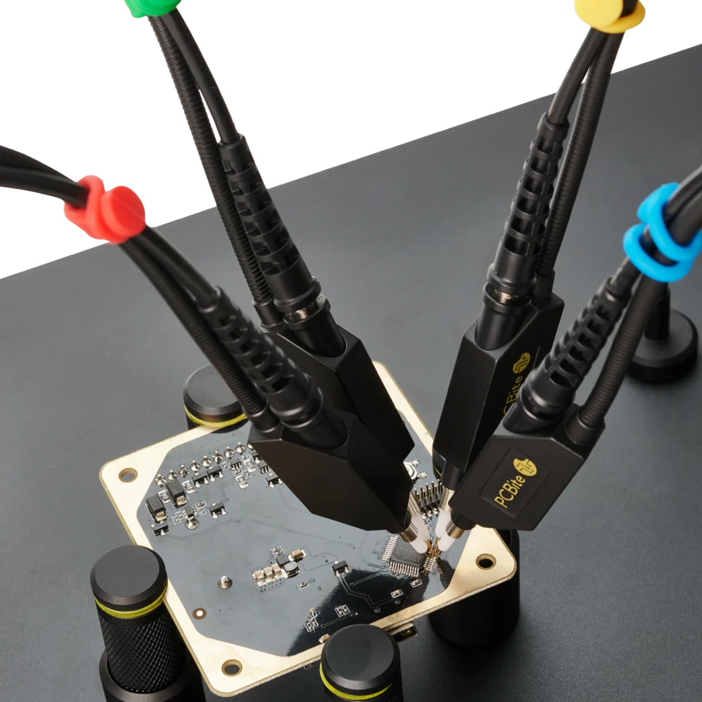
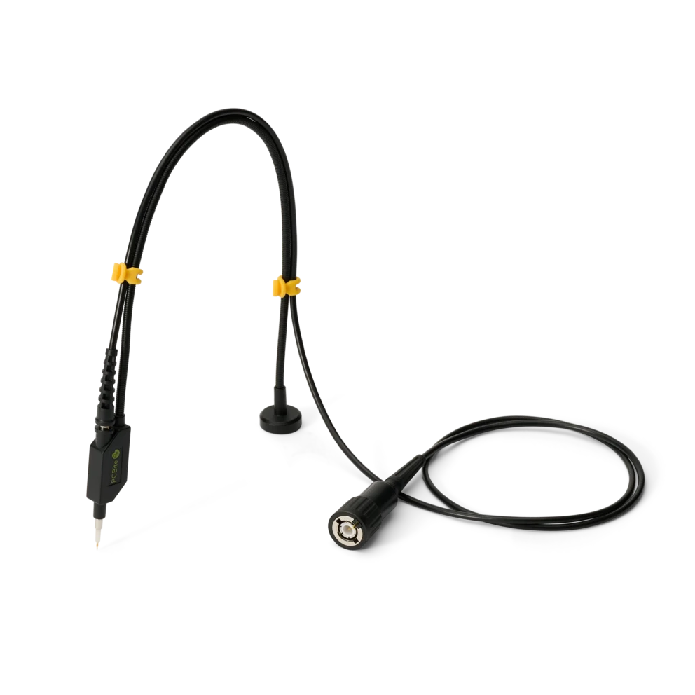
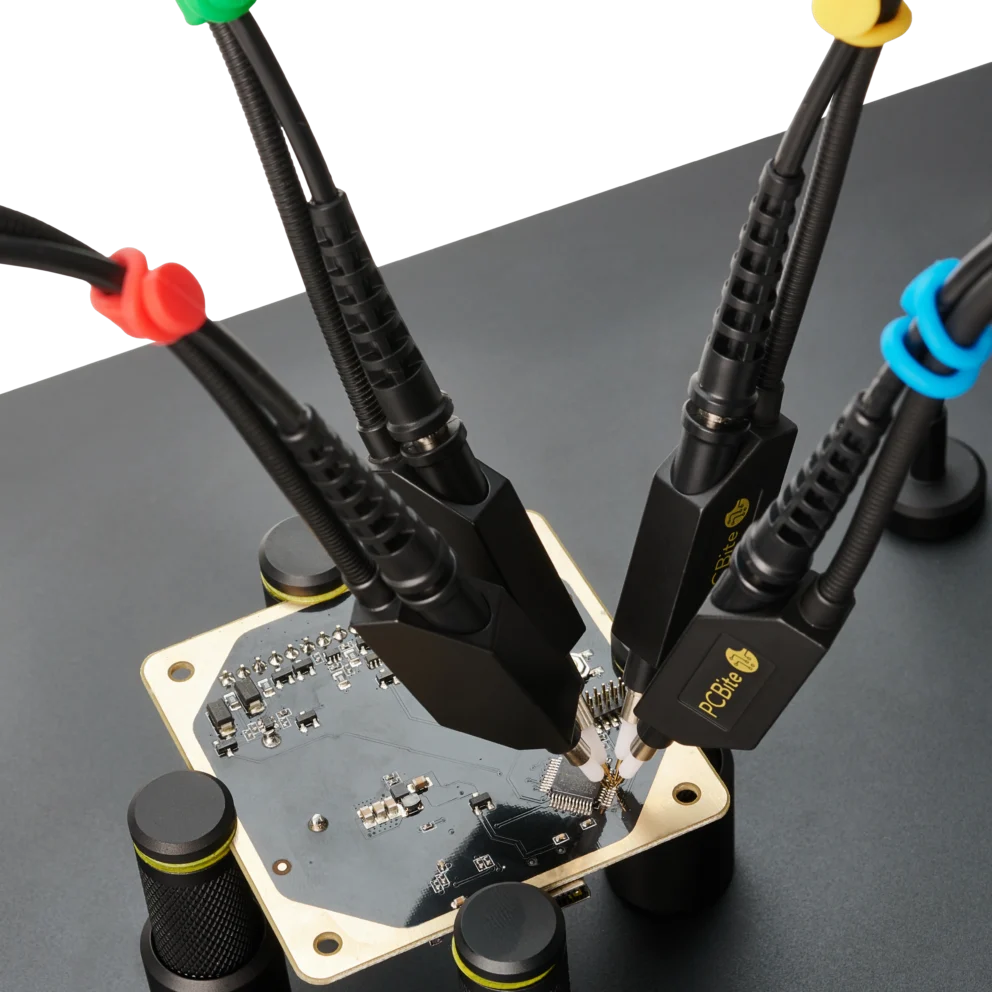
The PCBite SQ100, SQ200, SQ350 and SQ500 are 10:1 handsfree oscilloscope probes for 100 MHz to 500 MHz with 10 MΩ and 9 pF to 13 pF at the tip13. Sensepeek’s patented spring-loaded ground keeps the ground path short while the probe stays on the test point.
A logic analyzer compares each input with a threshold and records ones and zeros on many channels at once, then decodes I²C, UART and SPI into bytes. Choose the logic setting that matches the supply, for example 1.8 V or 3.3 V. The analyzer then switches at about half the supply, 0.9 V or 1.65 V14. Sample at least four times faster than the fastest signal, or the SPI clock15. A mixed signal oscilloscope (MSO) adds the same digital channels and protocol decoding to an oscilloscope, time-correlated with the analog channels16. Decode on the digital channels, trigger on the bad byte and look at the analog edge in the same capture.
The PCBite SP10 and SQ10 are 1:1 handsfree probes for logic analyzers and MSO digital channels17. They connect with 2.54 mm (0.100 in) jumper connectors, often called Dupont connectors, and hold a needle on each test point, so a full SPI bus with clock, data and chip select can be captured without soldering. With the included 0.8 m (31 in) test cables the SP10 and SQ10 are rated for signals up to 10 MHz. This is a practical limit set by the cables, not by the probes. At 20 nH to 25 nH per inch18, 19, a 0.8 m wire and the 10 pF input of a typical logic analyzer20 resonate at roughly 55 MHz to 65 MHz, near the fifth harmonic of a 10 MHz clock. Shorter cables move the resonance higher. For faster SPI clocks, use shorter cables or check the edges with an SQ oscilloscope probe.
Keep the cable lengths equal. Every cable delays the signal, by roughly 5 ns per metre. When a logic analyzer decodes a bus, it compares the edges on several lines, for example the data on MOSI with the clock edge on SCLK. If one line runs through a longer cable or a different kind of probe, its edges arrive later than the others. At higher clock rates the decoder can then read the data on the wrong side of the clock edge and show bytes that were never sent. A 50 cm difference adds about 2.5 ns: little on a 1 MHz bus, but a quarter of the time between the clock edge and the next data change on a 50 MHz SPI clock.
Use the same cable length for every signal on the bus. SP10 and SQ10 probes can be mixed on the same bus with the test wires that come with them, but do not mix cable lengths, and do not mix oscilloscope probes with SP10 or SQ10 probes on signals that are decoded together. On an MSO, decode on the digital channels, and use the oscilloscope’s deskew function when you compare an analog edge with a digital one.
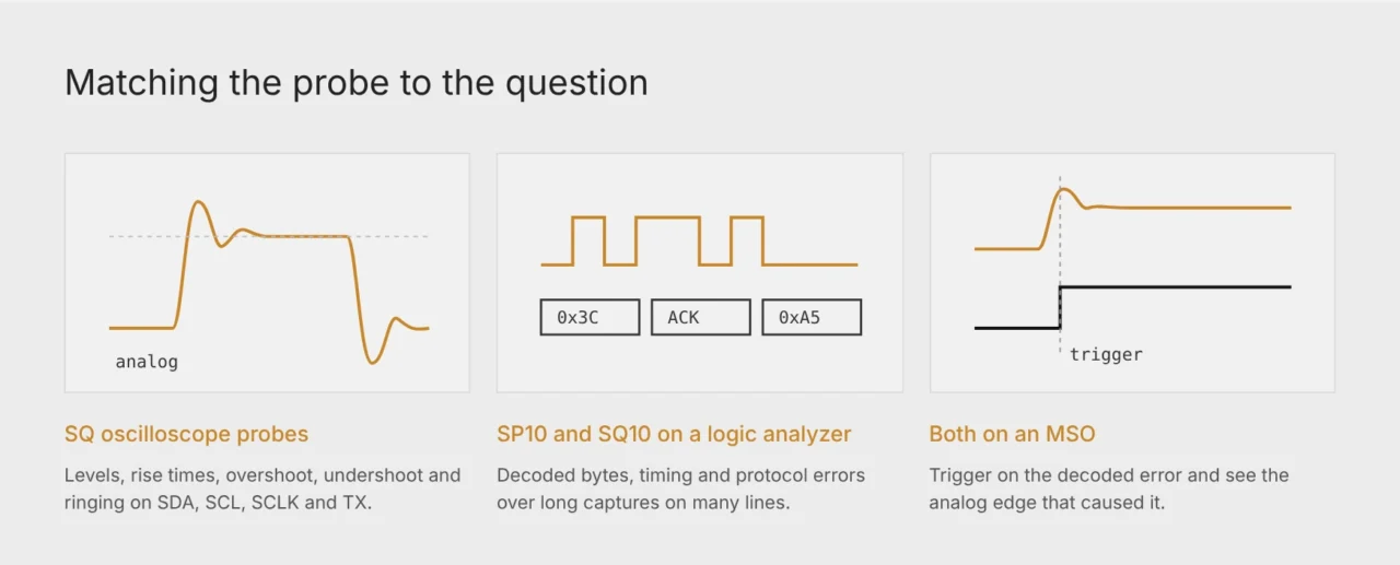
Fig. 4. The oscilloscope answers analog questions, the logic analyzer answers timing and protocol questions.
SQ oscilloscope probes for signal quality, SP10 and SQ10 for protocol decoding.
Du använder en föråldrad webbläsare. Alla funktioner fungerar inte i din webbläsare. Var vänlig uppgradera din webbläsare för att förbättra din upplevelse och öka din säkerhet.